Regions for Set Inclusion
Published April 3, 2026 · Revised July 24, 2026
Common distance- and transformation-based point embeddings do not encode set inclusion as a primitive: there is no geometric sense in which Dog is inside Animal rather than close to it. Axis-aligned box embeddings make intersection exact and supply a conditional-overlap score, but disjoint hard boxes have zero intersection volume and therefore zero gradient. Gumbel boxes make endpoint intersections closed in distribution and expected volumes smooth; their practical probability calculation still uses explicit approximations.
The claim that a dog is an animal is a statement about sets: every dog is an animal, so the set of dogs is contained in the set of animals. A model may learn a point-based score correlated with that relation, but ordinary point geometry does not make inclusion literal. Region representations can make inclusion literal.
Five questions recur, and a result about one does not settle the others:
| Question | What must be shown |
|---|---|
| Semantics | Which set relation the geometry is meant to represent |
| Representation | Which operations remain exact inside the chosen region family |
| Optimization | Whether the loss supplies useful gradients where training visits |
| Query composition | Whether projections, conjunctions, unions, and negations are exact or learned |
| Logical faithfulness | Whether geometric satisfaction matches the source theory’s consequences |
The article first builds containment and intersection as representation operations, then addresses the optimization failure of hard boxes. Query2Box and EL⁺⁺ are later, parallel applications: one composes answer-set queries, while the other scores normalized ontology axioms.
# Background
# Knowledge graph embeddings
A knowledge graph is a collection of triples : head entity, relation, tail entity. (“Berlin”, capitalOf, “Germany”) or (“Dog”, isA, “Animal”). These graphs are large but sparse: when Freebase was active, 71% of people had no recorded birthplace and 75% had no recorded nationality (West et al., 22). One frequently studied task is link prediction: given (Berlin, capitalOf, ?) or (?, isA, Animal), rank the missing entity.
Many approaches since 2013 embed entities as vectors and score triples geometrically: either by treating relations as transformations (TransE, RotatE) or as bilinear forms like where is a learnable matrix per relation (DistMult, ComplEx).The point-embedding models discussed here are implemented in tranz, named after the Trans* family (TransE, TransR, TransH, TransD). They can learn useful scores for hierarchical triples, but their native geometric operation is not set containment. The region embeddings that follow are in subsume, named for the subsumption relation ().
TransE 2, short for “translating embeddings,” models each relation as a translation: score a triple by .Lower scores indicate a closer fit. Implementations commonly use either an L1 or L2 norm. If the triple is true, the head plus the relation vector should land near the tail. Its small parameterization and inexpensive score made it a widely used baseline.
Under the exact translation equations, TransE degenerates on some one-to-many
and symmetric relations. For (Britain, hasCity, ?), each correct tail would
satisfy , forcing London, Manchester, and Edinburgh to the same point.
For a symmetric pair, and imply . Margin-based training
relaxes these equalities, but it does not make either relation pattern native
to the translation geometry.
RotatE 7, short for “rotation embedding,” fixes the symmetry problem by working in complex space: each relation is an element-wise rotation where . A symmetric relation requires , so each component can have phase or . This handles symmetry, antisymmetry, inversion, and composition.
Neither TransE nor RotatE makes containment a native geometric
operation.A learned distance score can rank hierarchical
triples successfully. What it does not supply is literal set inclusion:
“close to Animal” and “inside Animal” are different geometric statements. Both embed each entity as a point. A point has no volume,
interior, or boundary of its own, so one entity’s representation cannot be
inside another’s.
# What containment requires
Consider the subsumption hierarchy: Dog Animal LivingThing, where (read “is subsumed by”) means every instance of the left concept is also an instance of the right. In set-theoretic terms, where is the set of individuals that fall under concept .
An embedding that captures this needs three properties:
-
Volume. More general concepts (Animal) should have larger representations than specific ones (Dog). “Animal” covers more ground than “Dog.”
-
Containment. The representation of Dog should be geometrically inside the representation of Animal. Not just “close to,” but inside.
-
Intersection. The concepts “Animal” and “Pet” overlap (some animals are pets, some aren’t). Their representations should intersect, and the intersection should itself be a valid representation, of the concept , whether or not that conjunction has a name in the ontology.
Points do not supply these region operations. Order embeddings instead encode the partial order directly.
# Order embeddings
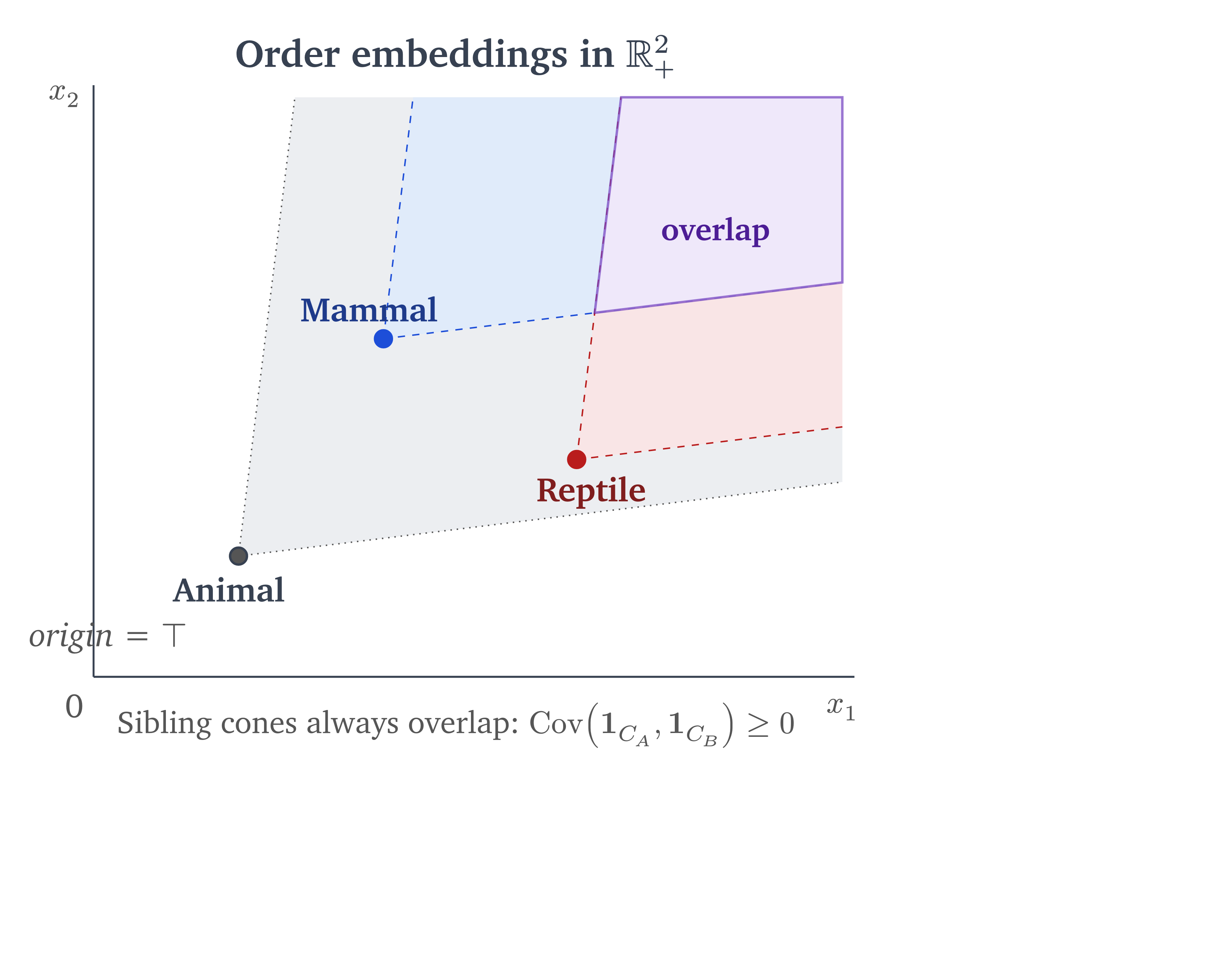
Vendrov et al. 3 embedded the partial order directly into the geometry. Their approach mapped concepts into the non-negative orthant (the region where all coordinates are , the -dimensional analogue of the first quadrant) and imposed the reverse product order: is more general than if for every coordinate. The origin is the top element, the most general concept.The “entity” concept, containing everything, sits at zero. Specificity grows with coordinate magnitude. Each point defines two cones: the cone extending toward the origin (smaller coordinates) contains its ancestors (more general concepts); the cone extending away from the origin (larger coordinates) contains its descendants (more specific concepts).
Reproduce this figure
The coordinate order is transitive: if and coordinate-wise, then . The representation is still points, and the cones are unbounded. Vilnis et al. 4 proved a limitation: for any product probability measure over the non-negative orthant, the covariance of the indicator functions of any two cones is non-negative, . If “Mammal” and “Reptile” are both under “Animal,” the model cannot make them negatively correlated or disjoint under that product measure.
The forced positive covariance between sibling cones motivated boxes: bounded regions closed under intersection, with a conditional-overlap containment score.
# Box Embeddings
Reproduce this figure
typst compile box_taxonomy.typ box_taxonomy.png --ppi 500 --root ..The idea of representing words as regions rather than points goes back to Erk 1, who embedded words as convex regions in vector space to model graded entailment. Vilnis et al. 4 adapted the idea to knowledge graphs with axis-aligned hyperrectangles, boxes, in . A box is parameterized by its minimum and maximum corners:
where and with for each coordinate.
One region family supporting all three properties is the axis-aligned box. Volume is the product of side lengths:
Containment is coordinate-wise: if and only if and for all . The intersection of two boxes is a box (or empty):
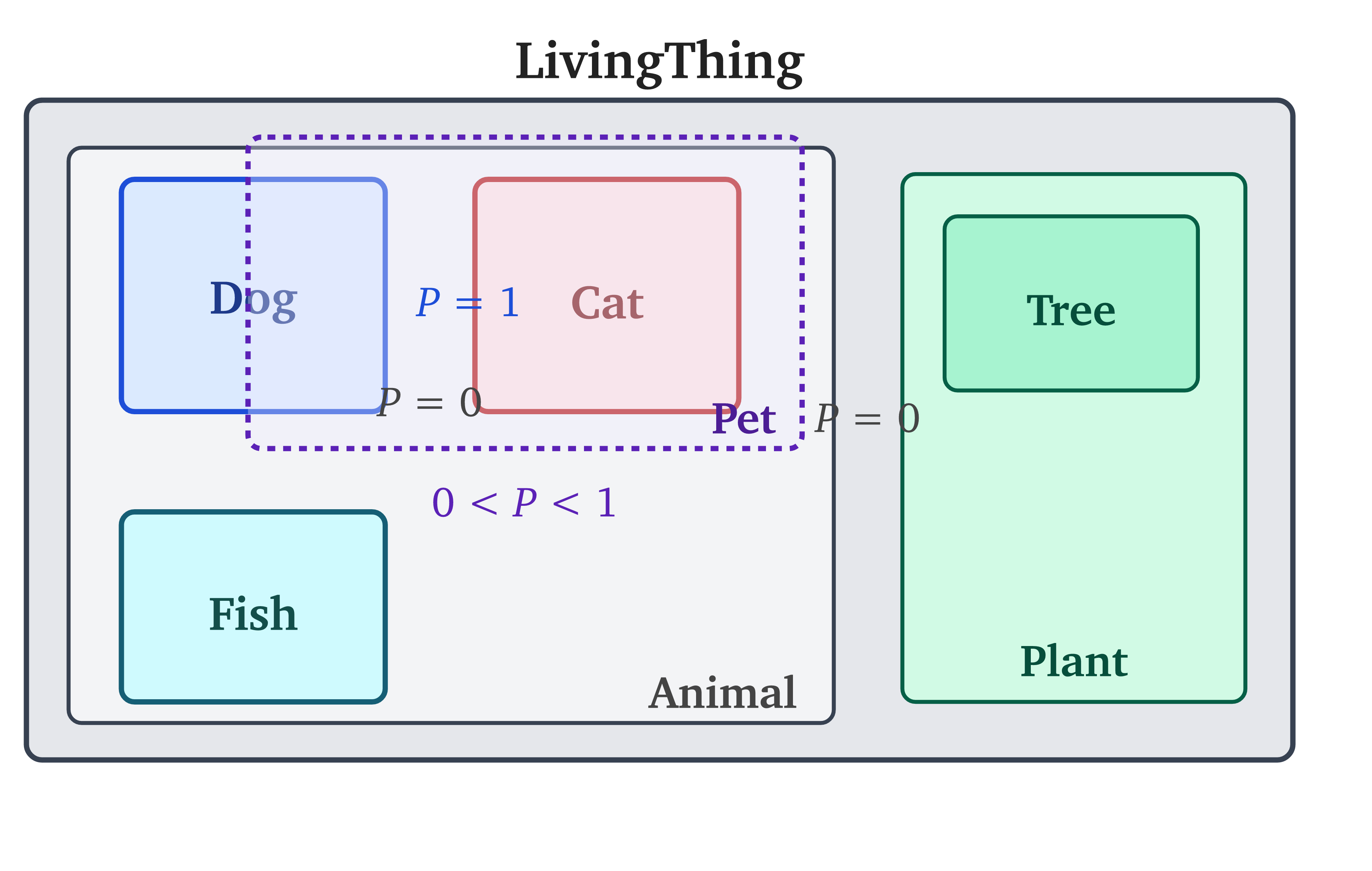
The intersection is non-empty when for every coordinate. If any coordinate has an empty interval, the boxes are disjoint. Disjoint boxes represent mutually exclusive concepts, the thing order embeddings could not express. And when boxes partially overlap, the intersection region is itself a box representing the conjunction: the box for “Animal” intersected with the box for “Pet” gives a box for “things that are both animals and pets.”
The axis-alignment is a deliberate restriction.The intersection of two balls is generally a lens rather than a ball. ELEmbeddings (Kulmanov et al., 2019), which used n-balls for EL⁺⁺ concepts, therefore approximated conjunction (, NF2 in Box²EL’s numbering). Boxes instead keep intersections in the same family. Rotated boxes would be more expressive, but their intersection is not necessarily a rotated box, so they lose that closure. Axis-aligned boxes ordered by inclusion form a lattice: their meet is intersection and their join is the smallest axis-aligned bounding box containing both. That join generally contains points not in the set union, so lattice closure should not be confused with exact closure under logical disjunction. Each dimension contributes an independent “vote” on containment, the box analogue of diagonal covariance.
# Conditional overlap
The geometric intuition is that a broad concept (Animal) gets a large box and a narrow concept (Labrador Retriever) gets a smaller box inside it. When training makes the inclusion constraints hold, volume becomes a model-side proxy for generality: a subset cannot have greater volume than its superset. The converse does not hold; a large box is not, by size alone, semantically general.
One score for subsumption is the fraction of covered by :
Concretely: draw a point uniformly from and ask whether it lands in . The event itself is deterministic; the ratio is not the probability that one fixed set contains another. It returns 1 if is entirely inside , 0 if they are disjoint, and an intermediate value for partial overlap. To express “Dog is-a Animal,” train toward 1.
The asymmetry is important: in general because the denominator changes. A small box inside a large box gives 1 in one direction and a small score in the other. This matches the semantics: every dog is an animal, but not every animal is a dog.
# A worked example
Take . Let Animal and Dog .
The intersection is Dog itself (Dog is inside Animal), so .
Now add Cat . Dog and Cat are disjoint (no overlap in the first coordinate: Dog’s doesn’t intersect Cat’s ), so . Both are contained in Animal. The geometry directly encodes the taxonomy.
import numpy as np

def conditional_overlap(a_min, a_max, b_min, b_max):
    """Fraction of B's volume covered by A."""
    inter_min = np.maximum(a_min, b_min)
    inter_max = np.minimum(a_max, b_max)
    inter_sides = np.maximum(inter_max - inter_min, 0)
    b_sides = np.maximum(b_max - b_min, 1e-10)
    return np.prod(inter_sides) / np.prod(b_sides)

animal = (np.array([0, 0]), np.array([10, 10]))
dog    = (np.array([2, 3]), np.array([5, 7]))
cat    = (np.array([6, 3]), np.array([9, 7]))

print(conditional_overlap(*animal, *dog))  # s(Animal | Dog) = 1.0
print(conditional_overlap(*dog, *animal))  # s(Dog | Animal) = 0.12
print(conditional_overlap(*cat, *dog))     # s(Cat | Dog) = 0.0
In high dimensions, computing the raw volume numerically is unstable: floating-point underflow to zero can occur before the full product is computed. Computing in log-space avoids that product: . Practical implementations commonly use log-volumes for this reason.
# The Gradient Problem
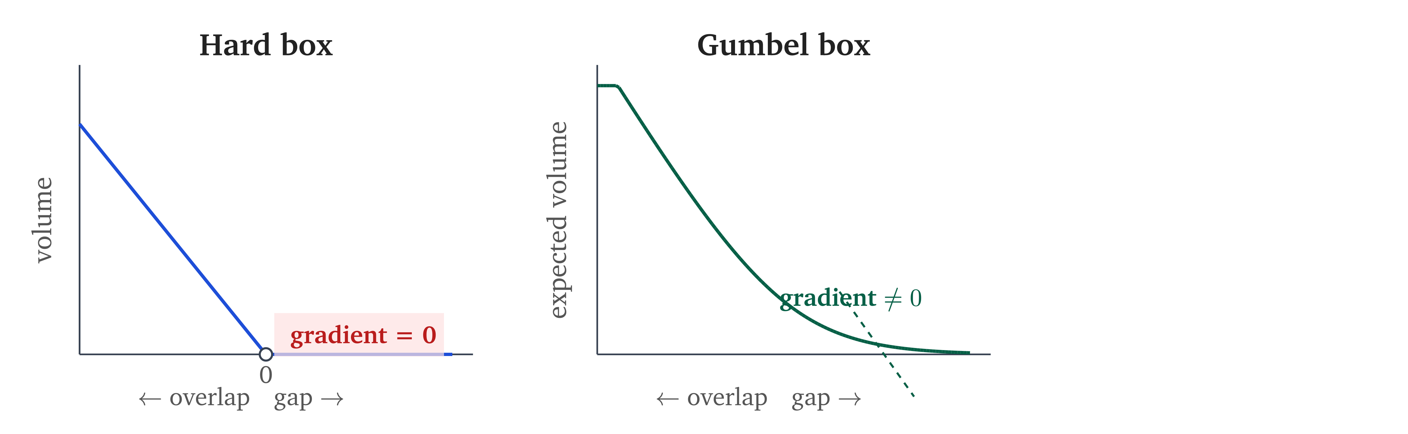
Hard overlap-volume objectives have zero-gradient regions.When many pairs initialize disjoint, a naive overlap-volume objective can stall because those pairs supply no local direction of improvement. Consider two disjoint boxes – say Dog and Fish . Their intersection volume is zero. If we move Dog slightly – say shift it by in any direction – the intersection is still zero. The loss doesn’t change. The gradient is zero.
Dasgupta et al. call this a local identifiability problem.In their definition, parameters are locally identifiable when every sufficiently small distinct perturbation changes the likelihood. Flat overlap-volume neighborhoods violate that criterion. The operational fact used here is the flat score, not a claim that every box-model parameter is globally unidentifiable. When boxes are disjoint, the containment probability is identically zero in a neighborhood of the current parameters. The optimizer receives no signal about which direction to move to bring the boxes closer.
The problem gets worse in high dimensions. In , two boxes are disjoint if any single coordinate has non-overlapping intervals. If independently initialized intervals overlap in one coordinate with probability , then all coordinates overlap with probability . The exact value depends on the initialization law, but the exponential dependence on makes fully overlapping random pairs scarce in high dimensions.
The intersection volume is piecewise multilinear in the box coordinates. Within each combinatorial regime (fully contained, partially overlapping, disjoint), it is a product of linear terms, one per coordinate. The containment probability, as a ratio of two such products, is a piecewise rational function. At the boundaries between regimes, the function is continuous but not differentiable. And in the disjoint regime, it is flat: identically zero, with zero gradient everywhere.
The failure mode is analogous to the dead ReLU problem in neural networks, but the mechanism differs. A dead ReLU neuron produces zero gradient for its current input but can recover if the bias shifts enough to re-enter the positive region. Here the problem is gradient sparsity at initialization: in high dimensions, almost every pair of boxes starts disjoint, so almost every training signal is zero. The gradient doesn’t die during training – it was never there to begin with. A dead ReLU affects one neuron; this affects all parameters of every disjoint pair simultaneously.
Reproduce this figure
typst compile gradient_landscape.typ gradient_landscape.png --ppi 500 --root ..# First fix: smoothing (Li et al., 2019)
Li et al. 6 addressed the gradient problem by convolving the hard box indicator functions with Gaussian kernels. The smoothed intersection is never exactly zero; even for disjoint boxes, the Gaussian tails overlap, providing gradient signal.
The smoothed volume has a closed-form expression involving the Gaussian CDF, which is differentiable everywhere. This works: disjoint boxes now produce nonzero loss, and the optimizer can move them toward overlap.
The smoothed membership family is not closed under exact pointwise conjunction: multiplying two Gaussian-smoothed box indicators does not in general produce another member of the same parameterized family. That is a different statement from saying the underlying hard-box order vanished; the SmoothBox paper explicitly retains useful lattice properties. In the one-dimensional balanced-tree experiment reported by Dasgupta et al. 8, SmoothBox reached MRR 0.691 and Gumbel boxes 0.971. The paper attributes the gap to local identifiability and optimization. It is an empirical result in that setting, not a proved expressivity ceiling caused by “loss of lattice.”
# Second fix: Gumbel boxes (Dasgupta et al., 2020)
Dasgupta et al. 8 use an endpoint family whose min/max operations remain closed in distribution.
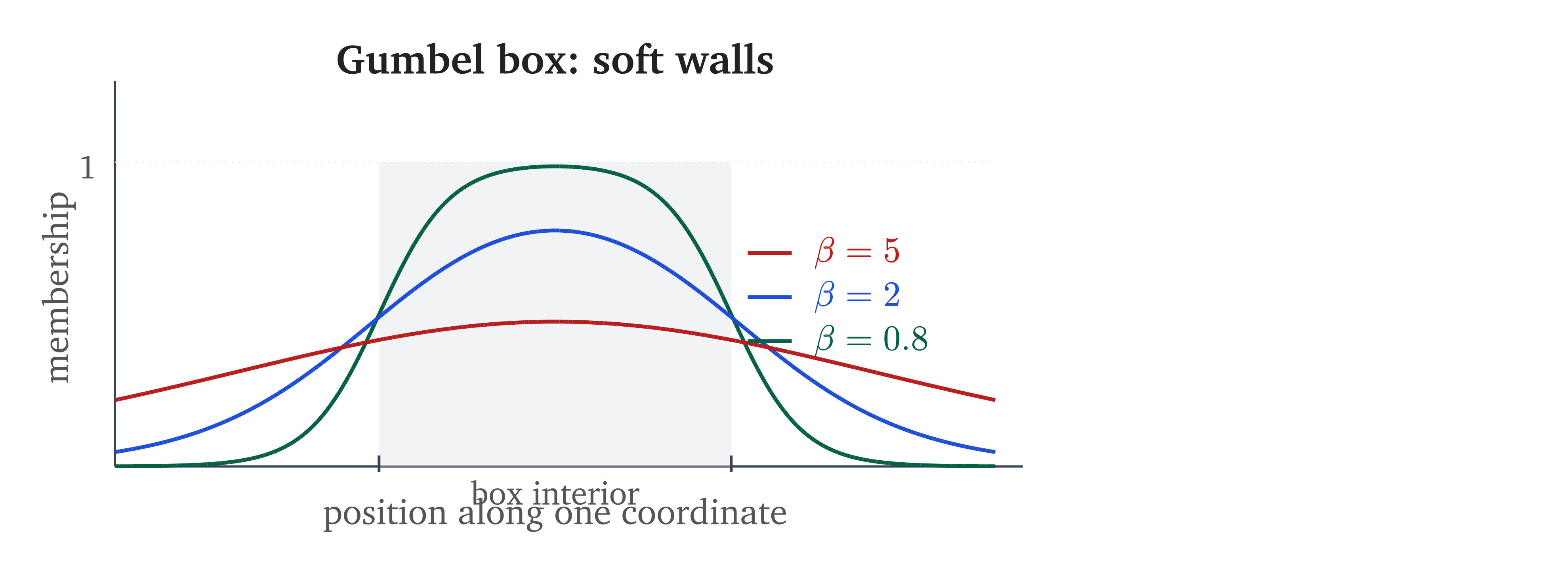
Instead of a deterministic box , make each endpoint a random variable drawn from a Gumbel distribution. The Gumbel distribution appears as the limiting distribution of the maximum (or minimum) of many independent samples; it is to maxima what the Gaussian is to averages. It comes in two variants: Gumbel-max (right-skewed, models maxima) and Gumbel-min (left-skewed, models minima). The lower bound gets a Gumbel-max because box intersection takes the of lower bounds; the upper bound gets a Gumbel-min because intersection takes the of upper bounds.The pairing follows the intersection rule: the new lower bound is the maximum of the old lower bounds, while the new upper bound is the minimum of the old upper bounds.
where are learnable location parameters and is a temperature controlling the “softness” of the boundaries. At , the Gumbel distributions collapse to point masses and we recover hard boxes.One analogy is wall thickness: a larger spreads the boundary transition, while a smaller sharpens it.
Why Gumbel specifically, and not Gaussian or logistic or any other smooth distribution? The answer is visible from the Gumbel-max CDF
For independent equal-scale variables ,
where
The maximum is therefore another Gumbel-max variable, with its location updated by LogSumExp. Negating the variables gives the corresponding min-stability result. This is exactly the pair of operations needed for box intersection:
By the Fisher-Tippett-Gnedenko theorem, the only max-stable distribution families are Gumbel, Fréchet, and Weibull, so stability is not unique to Gumbel. The Gumbel construction combines it with the LogSumExp location above and a tractable expected-length integral.
Recall that box intersection takes the coordinate-wise max of lower bounds and min of upper bounds. With Gumbel endpoints, the intersection of two Gumbel boxes is again a Gumbel box, computed in closed form via LogSumExp. This is exact closure of the endpoint distribution family; the expected-volume score built on top of it is approximated.
# Where the Bessel function comes from
The expected side length of a Gumbel box along one coordinate involves a modified Bessel function . What matters is its behavior: starts at infinity for argument zero, then drops off smoothly (monotonically decreasing, convex, and asymptotically ). For large positive gap between box endpoints (box is wide open), the expected volume is large. For (box is barely open), it is small but nonzero. For (endpoints are “inverted,” meaning the box is empty in expectation), it is tiny but still has a nonzero derivative . The optimizer retains a signal. Hard intersection volume lacks that signal; both SmoothBox and Gumbel boxes restore it with different constructions.
The formula: the expected side length is where is Gumbel-min and is Gumbel-max. Integrating the product of a Gumbel-max PDF and a Gumbel-min survival function gives:
where is the gap between the location parameters. In this calculation, a change of variables reduces the Gumbel endpoint integral to an integral representation of .
For a random Gumbel box, the conditional-overlap quantity is itself a random ratio. The practical Gumbel-box score replaces with the ratio of expected volumes . That is a deliberate tractable approximation, not an identity obtained from min/max stability.
A concrete comparison in 1D: two intervals that should overlap but are currently disjoint, with a gap of 2 units.
- Hard box: gradient zero everywhere. The optimizer has no direction.
- Softbox (): Gaussian tails give a nonzero gradient. In the paper’s 1D balanced-tree experiment, MRR reached 0.691.
- Gumbel box (): the expected side-length calculation also gives a nonzero gradient. In the same experiment, MRR reached 0.971.
Gumbel boxes do more than change the smoothing kernel: min/max-stable endpoints keep intersections in the same distribution family while expected side lengths remain differentiable. The implemented score then layers the ratio-of-expectations and softplus approximations above that exact closure.
# The softplus approximation
Computing Bessel functions in every forward pass is expensive. Dasgupta et al. 8 observed that is nearly indistinguishable from a shifted softplus, and proposed:
where is the Euler-Mascheroni constant. Appendix C of Dasgupta et al. 8 reports a numerically observed maximum error of about over . That is an empirical range check, not a proved global bound, and its practical effect depends on the surrounding loss and temperature.
The paper’s implementation uses this shifted softplus approximation. It is
differentiable, monotonic with respect to containment, and numerically stable.
The approximate expected volume is the product of the per-coordinate
lengths. Its log is therefore a sum of log-softplus terms, plus the scale
contribution , with the same linear-in- complexity as a hard
box.
The construction now has several layers that should not be collapsed:
| Layer | Status |
|---|---|
| Max of lower endpoints and min of upper endpoints | Exact closure for independent, equal-scale Gumbel endpoint families |
| Expected positive side length | Exact formula for independent, unconstrained endpoints |
| Expected volume as a product of side lengths | Uses independence across coordinates |
| Replacing a bounded domain by the unconstrained integral | Approximation |
Replacing the expression by shifted softplus |
Approximation |
| Replacing an expected volume ratio by a ratio of expected volumes | Approximation |
Reproduce this figure
typst compile gumbel_walls.typ gumbel_walls.png --ppi 500 --root ..The temperature can also be used as a curriculum: an implementation may start with softer boundaries and anneal toward a smaller value. That is a training strategy, not a requirement of the Gumbel-box derivation.
Gumbel boxes retain the union and complement limitations of hard boxes. Exact interval union would require the minimum of lower endpoints and maximum of upper endpoints, which are not the stable operations for the chosen endpoint families; a disjoint union is not one interval in any case. The complement of a Gumbel box is not a Gumbel box. Their contribution is differentiable expected volume while preserving the supported intersection operation.
# Query2Box: Answering Logical Queries
The first application branch asks whether boxes can do more than subsumption.
Ren et al. 9 introduced Query2Box (the name
says it: translate a logical query into a box), applying box embeddings to
multi-hop logical queries over knowledge graphs. It uses learned query
operators rather than the Gumbel expected-volume construction: represent a
query as a box, then rank answer entities by distance to that box.
Consider the query: “Where did Canadian Turing Award winners graduate?”This is the running example from Ren et al. 9, and it also appears in Stanford CS224W lectures. This decomposes into: start with TuringAward (a point), apply the “Win” relation projection to get a box of Turing winners, separately start with Canada, project via “Citizen” to get a box of Canadians, intersect the two boxes, then project via “Graduate” to get universities. Each relation projection translates the box center and adds to the box offset, so the box can grow but not shrink. This parameterization accommodates one-to-many relations by expanding the candidate region.
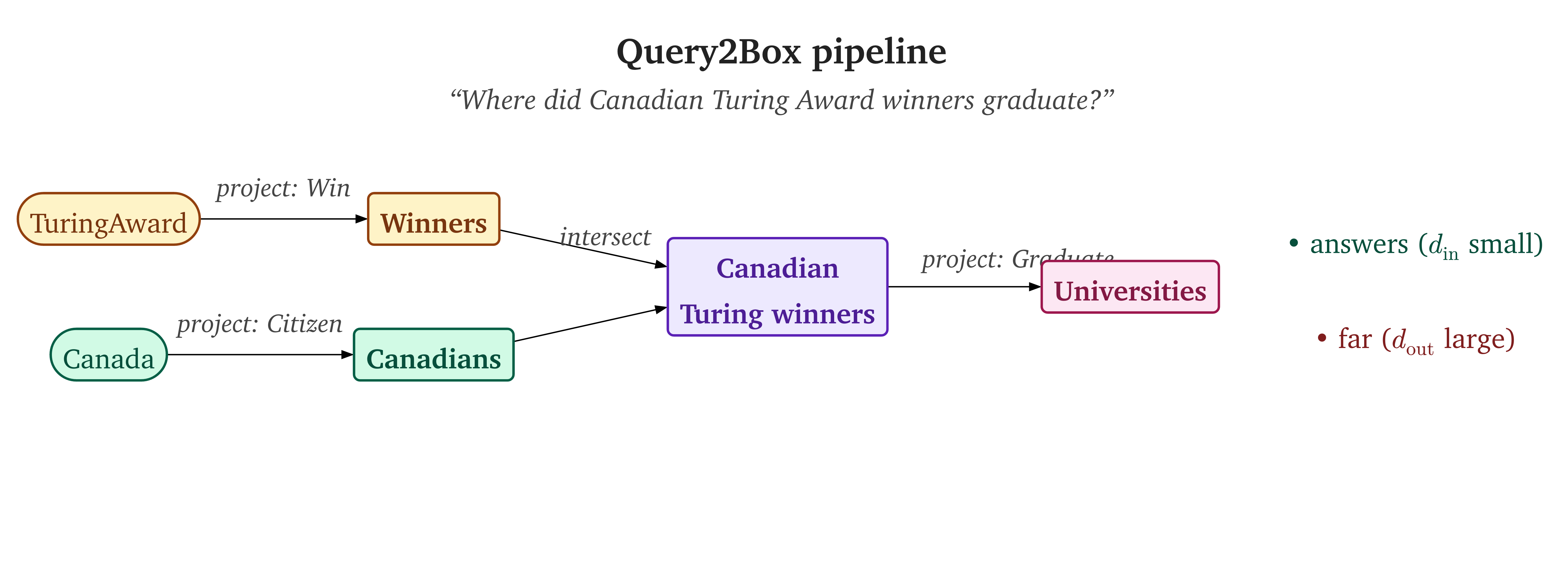
Reproduce this figure
typst compile query2box_pipeline.typ query2box_pipeline.png --ppi 500 --root ..Note the asymmetry: queries are boxes, but answer entities are still embedded as points.Query2Box uses points for candidate entities and boxes for queries; these representations serve different roles. The box represents the set of plausible answers; each candidate entity is a point that may or may not land inside it. The scoring function for a candidate answer entity (embedded as a point) relative to a query box is:
where is the L1 distance from to the box itself (zero inside), while measures the distance from the box center to the coordinate-wise clamp of into the box. For an inside point the clamp is ; for an outside point it is the nearest point in the box. The hyperparameter , set to in the original paper, downweights this center-to-clamp term.
The asymmetry between and is intentional. Outside entities should be penalized heavily (they are not answers to the query). Inside entities are all plausible answers, but we mildly prefer those closer to the center.
Intersection of query boxes models conjunction: “countries that border France and have population > 50M” corresponds to intersecting two query boxes. Recall that geometric intersection is coordinate-wise max of lower bounds, min of upper bounds. This works when boxes overlap, but after multiple projection steps the boxes may not overlap at all, and an exact empty intersection gives zero volume with zero gradient (the same dead-zone problem from the previous section). Query2Box sidesteps this with a learned intersection operator: an attention mechanism over the input boxes’ centers produces the new center, combined with a coordinate-wise minimum of offsets to shrink the box. This is an approximation, not a geometric intersection, but it provides gradient signal in all configurations.
Two operations that boxes cannot handle:
Union. The union of two boxes is generally not a box. Query2Box works around this by transforming queries into disjunctive normal form (DNF): push all disjunctions to the last step, compute each conjunctive branch as a box, then aggregate scores across branches.DNF means rewriting the query so all ORs are at the outermost level. Each branch is a pure conjunction, representable as a single box. This is sound but adds computational cost proportional to the number of disjuncts.
Negation. The complement of a box in is an unbounded region that is not a box. Queries like “European countries that do not border France” require a different approach. This limitation motivated two lines of follow-up work: geometric alternatives (cones) and algebraic alternatives (fuzzy logic).
# Beyond Boxes: Cones and Negation
Zhang et al. 12 introduced ConE (“cone embeddings”), which represents a query in dimensions as a Cartesian product . Each is a sector-cone on a circle, parameterized by an axis angle and an aperture angle.
The exact operation ConE gains is a particular negation: the closure-complement of a sector-cone is representable by flipping its axis and aperture. Ordinary set complement differs on the boundary. Intersections of sector-cones are not always sector-cones, so ConE learns a neural intersection approximation; the paper reports mean intersection Jaccard 0.6134 over 8,000 randomly sampled pairs of sector-cones.12 Union is handled after DNF as a set of branch cones, not collapsed to one cone.
Cones also have no finite volume, so they lack the finite-measure conditional score that boxes provide. That does not make box scores automatically calibrated: calibration is an empirical property to test with reliability curves, Brier score, or log loss. The geometries support different operations; neither one wins by definition.
BetaE 10 embeds queries as Beta
distributions. Its learned negation operator maps each parameter pair by
reciprocal, . The t-norm fuzzy logic
approach 11 13 decomposes complex queries into atomic link
predictions aggregated with continuous AND/OR operators, without requiring
training examples of the full complex queries.
# EL⁺⁺ and Ontology Completion
The second application branch returns to subsumption, but now asks how region constraints correspond to a formal ontology. Biomedical ontologies including SNOMED CT, Gene Ontology, and GALEN contain large fragments that can be normalized into lightweight description logics in the EL family. Embedding benchmarks often use an EL⁺⁺ normalization, a fragment of first-order logic designed for efficient reasoning.The source ontologies are not all written in exactly the same fragment. The benchmark normalization is the relevant object here. A classical reasoner derives logical consequences; an embedding model assigns scores that may be useful for ranking held-out or candidate axioms. EL⁺⁺ allows concept conjunction (), existential restriction (, “things that have an -relationship to some ”), and a bottom concept (). A central inference is subsumption: given an ontology, determine whether holds (every instance of is an instance of ).
Classical reasoners (ELK, Snorocket) compute subsumption exactly by rewriting the ontology’s axioms into normal forms: standardized shapes like or that decompose complex axioms into restricted forms. This is complete for logical entailment but does not rank plausible, unentailed subsumptions; embedding methods are used for that ranking task.
Jackermeier et al. 16 developed Box²EL
(“dual box embeddings for EL”). It represents each role with a head box
and a tail box , and gives
each atomic concept a learned translation vector
. The bump vectors let the role constraint depend on
the concepts at both ends. Its geometric losses cover the four concept and
existential forms below, along with separate losses for disjointness and role
inclusions. The numbering here follows the Box²EL paper; some implementations,
including subsume, swap NF1 and NF2.
NF1: . Direct subsumption. “Pneumonia ⊑ Disease-of-Respiratory-System” – every pneumonia is a respiratory disease. The Pneumonia box should sit inside the Disease-of-Respiratory-System box. In center-offset parameterization (storing a box as its midpoint and half-widths instead of min/max corners), define:
Each coordinate is the larger one-sided boundary excess. Exact containment means for every coordinate; the components need not equal zero. If centered box is wider than by , then protrudes by on each side and . One implementation-level loss is:
With , the loss is zero exactly when is contained in . A positive tolerates up to of protrusion per coordinate; a negative value requires clearance inside . Calling a margin does not by itself say which behavior is intended – its sign does.
NF2: . Conjunction implies subsumption. “Inflammation ⊓ Lung-Disorder ⊑ Pneumonia” – things that are both inflammatory and lung disorders are pneumonia. The intersection of the Inflammation box and the Lung-Disorder box should fit inside the Pneumonia box.
NF3: . Existential restriction. “Pneumonia ⊑ ∃hasLocation.Lung” – every pneumonia has a location, and that location is a lung. Box²EL requires both
NF4: . Inverse restriction. “∃causedBy.Bacterium ⊑ Bacterial-Infection” – anything caused by a bacterium is a bacterial infection. In Box²EL, the possible sources connected to by lie within , so the loss requires
The Box²EL evaluation compares against the ontology-embedding methods ELEm, EmEL⁺⁺, BoxEL, and ELBE on held-out subsumption axioms from GALEN, Gene Ontology, and Anatomy. The paper reports a median rank about 60% below the next-best method on GALEN, more than 80% below it on Gene Ontology, and more than 40% below it on Anatomy.16 These are results under that paper’s data splits and protocol, not a comparison with classical deductive reasoning.
# Volume as an order constraint
If the learned boxes satisfy , then automatically. Along a correctly represented taxonomy, descendants therefore cannot be larger than their ancestors. This is a consequence of containment, not evidence that volume alone recovers semantic depth: unrelated concepts can have any relative volumes, and approximate training may violate the intended inclusions.
# Geometry Choices
The region-embedding literature developed along several connected lines: probabilistic boxes, multi-hop query answering, and ontology embeddings.
| Year | Model | Geometry | Subsumption signal | Conjunction | Negation |
|---|---|---|---|---|---|
| 2009 | Regions (Erk) | Convex regions | Volumetric | Exact convex intersection | Not in-family |
| 2013 | TransE (Bordes) | Point + translation | Learned distance | Not a region operation | Not a region operation |
| 2018 | Box Lattice (Vilnis) | Axis-aligned boxes | Conditional overlap | Exact intersection | Not in-family |
| 2018 | Entailment Cones (Ganea) | Hyperbolic cones | Geodesic order | Geometry-specific | Not supplied |
| 2019 | SmoothBox (Li) | Smoothed boxes | Soft volumetric | Not exact in-family | Not in-family |
| 2020 | Gumbel Box (Dasgupta) | Random-endpoint boxes | Approximate expected-volume ratio | Endpoint family exact | Not in-family |
| 2020 | Query2Box (Ren) | Query boxes | Point-to-box distance | Learned operator | Not supplied |
| 2020 | BetaE (Ren) | Product of Beta distributions | KL divergence | Learned operator | Reciprocal parameters |
| 2021 | ConE (Zhang) | 2D angular sectors | Angular distance | Learned operator | Exact closure-complement |
| 2021 | CQD (Arakelyan) | Link scores + fuzzy logic | Learned score | Chosen t-norm | Chosen fuzzy operator |
| 2022 | BoxEL (Xiong) | Boxes for EL⁺⁺ | Logical losses | Model-specific exact constraints | Not supplied |
| 2024 | Box²EL (Jackermeier) | Dual boxes for EL⁺⁺ | Logical losses | Model-specific exact constraints | Not supplied |
| 2025 | TransBox (Yang) | Boxes for EL⁺⁺ | Logical losses | EL⁺⁺-closed operations | Not supplied |
Sources for the comparison table
The rows summarize the primary papers in references 1–16, plus 20. “Exact” refers only to closure of the named representation under that operation; it does not claim exact recovery of the source theory.
No single geometry is best across these tasks.The
representation determines which operations can remain inside the model family;
the optimizer then determines how the chosen constraints are fitted. Ontology-embedding objectives translate normalized axioms into
geometric constraints, but zero loss guarantees only the conditions proved for
that model. A geometry does not, by itself, force all and only the logical
consequences of the source ontology. Graph-embedding approaches such as
TransE and RotatE instead optimize scores on triples and do not supply a
logical-model guarantee.
For subsumption-only tasks where inclusion is the chosen semantics, boxes or Gumbel boxes are a suitable model family; that choice does not by itself guarantee faithful ontology completion. Queries requiring negation or disjunction need an additional representation or decomposition, such as cones, DNF branches, or fuzzy operators. Hyperbolic cones (Ganea et al., 5) are the main alternative to boxes for hierarchies – hyperbolic space is a “continuous tree” where volume grows exponentially with radius, but a DAG with several independent parent chains is harder to place faithfully in one tree-like metric.Nickel & Kiela’s Poincaré embeddings (2017) do handle WordNet, which is a DAG. The limitation is not “DAGs are impossible”; it is that several unrelated hierarchies must share one metric geometry. Chami et al. (2020, MuRP) address relational variation with relation-specific parameters. Boxes can represent intersections directly: “things that are both mammals and flying creatures” is the overlap of two regions.
# Open Problems
Convexity. Helly-type intersection constraints impose real expressivity limits, but the statement depends on the region family and rule language. For ordinary axis-aligned boxes, pairwise intersection implies a common intersection because the intervals overlap in every coordinate. General convex sets in instead have Helly number , not 2. In a region-based rule setting, Charpenay and Schockaert 15 construct consistent combinations of hierarchy, intersection, and mutual-exclusion rules for which every convex embedding also satisfies an unintended hierarchy rule. That is a concrete counterexample to universal expressivity; it is not a claim that every ontology with multiple intersections is unrepresentable.
Faithfulness. Box embeddings can approximate but may not perfectly represent
the logical structure of an ontology. BoxEL proves a local guarantee about
its loss design: when the loss for an encoded axiom is zero, that axiom is
satisfied by the induced geometric interpretation.14 This does not prove that every candidate
subsumption scored by the model is entailed by the source ontology, nor that
every entailed subsumption receives zero loss. Those are stronger
no-extra-consequences and completeness requirements. TransBox (Yang et al.,
20) keeps more EL⁺⁺ operations inside its
representation and proves soundness properties, but not strong faithfulness for
full EL⁺⁺.
FaithEL (Lacerda, Ozaki & Guimarães, 21) proves that normalized ELH has a strongly
faithful convex embedding: the geometry can capture exactly the ontology’s
consequences in that fragment. Extending comparable guarantees to richer
role-composition settings remains an open direction. A pragmatic alternative,
DELE (Mashkova et al., 17), computes
deductive closure with a classical reasoner and uses it to train and evaluate
the embedding without treating entailed statements as negatives.
Evaluation methodology. Negative-sampling protocols can draw axioms that are
not asserted but are logically entailed, thereby penalizing a model for a true
consequence. DELE 17 computes the
deductive closure and
filters it from the negative set. Papers also use different data splits and
metrics, so cross-paper numerical comparisons require care.
Beyond axis-alignment. Axis-aligned boxes assume that dimensions are independent: the containment of Dog within Animal decomposes into independent interval containments. Octagons (Charpenay and Schockaert, 15) partially address this by adding diagonal constraints at cost . Full covariance (oriented boxes, ellipsoids) would be more expressive, but the intersection of oriented boxes is not an oriented box. None of the practical families surveyed here is closed under intersection, union, complement, and projection.
# References
[1] Erk, K. (2009). “Representing Words as Regions in Vector Space.” CoNLL, 57–65. ↩
[2] Bordes, A., Usunier, N., Garcia-Duran, A., Weston, J. & Yakhnenko, O. (2013). “Translating Embeddings for Modeling Multi-relational Data.” NeurIPS, 2787–2795. ↩
[3] Vendrov, I., Kiros, R., Fidler, S. & Urtasun, R. (2016). “Order-Embeddings of Images and Language.” ICLR. ↩
[4] Vilnis, L., Li, X., Murty, S. & McCallum, A. (2018). “Probabilistic Embedding of Knowledge Graphs with Box Lattice Measures.” ACL, 263–272. ↩
[5] Ganea, O.-E., Becigneul, G. & Hofmann, T. (2018). “Hyperbolic Entailment Cones for Learning Hierarchical Embeddings.” ICML. ↩
[6] Li, X. L., Vilnis, L., Zhang, D., Boratko, M. & McCallum, A. (2019). “Smoothing the Geometry of Probabilistic Box Embeddings.” ICLR. ↩
[7] Sun, Z., Deng, Z.-H., Nie, J.-Y. & Tang, J. (2019). “RotatE: Knowledge Graph Embedding by Relational Rotation in Complex Space.” ICLR. ↩
[8] Dasgupta, S. S., Boratko, M., Zhang, D., Vilnis, L., Li, X. L. & McCallum, A. (2020). “Improving Local Identifiability in Probabilistic Box Embeddings.” NeurIPS. ↩
[9] Ren, H., Hu, W. & Leskovec, J. (2020). “Query2Box: Reasoning over Knowledge Graphs in Vector Space using Box Embeddings.” ICLR. ↩
[10] Ren, H. & Leskovec, J. (2020). “Beta Embeddings for Multi-Hop Logical Reasoning in Knowledge Graphs.” NeurIPS. ↩
[11] Arakelyan, E., Daza, D., Minervini, P. & Cochez, M. (2021). “Complex Query Answering with Neural Link Predictors.” ICLR (Outstanding Paper). ↩
[12] Zhang, Z., Wang, J., Chen, J., Ji, S. & Wu, F. (2021). “ConE: Cone Embeddings for Multi-Hop Reasoning over Knowledge Graphs.” NeurIPS. ↩
[13] Chen, X., Hu, Z. & Sun, Y. (2022). “Fuzzy Logic Based Logical Query Answering on Knowledge Graphs.” AAAI. ↩
[14] Xiong, B., Potyka, N., Tran, T.-K., Nayyeri, M. & Staab, S. (2022). “Faithful Embeddings for EL⁺⁺ Knowledge Bases.” ECML-PKDD. ↩
[15] Charpenay, V. & Schockaert, S. (2024). “Embedding Ontologies with Octagons.” IJCAI. ↩
[16] Jackermeier, M., Chen, J. & Horrocks, I. (2024). “Dual Box Embeddings for the Description Logic EL⁺⁺.” WWW '24. ↩
[17] Mashkova, O., Zhapa-Camacho, F. & Hoehndorf, R. (2024). “DELE: Deductive EL⁺⁺ Embeddings for Knowledge Base Completion.” arXiv:2411.01574. ↩
[20] Yang, H., Chen, J. & Sattler, U. (2025). “TransBox: EL⁺⁺-closed Ontology Embedding.” WWW '25. ↩
[21] Lacerda, E., Ozaki, A. & Guimarães, R. (2024). “Strong Faithfulness for ELH Ontology Embeddings.” EKAW 2024. arXiv:2310.02198. ↩
[22] West, R., Gabrilovich, E., Murphy, K., Sun, S., Gupta, R. & Lin, D. (2014). “Knowledge Base Completion via Search-Based Question Answering.” WWW '14, 515–526. ↩