Is 561 Prime?

December 16, 2024

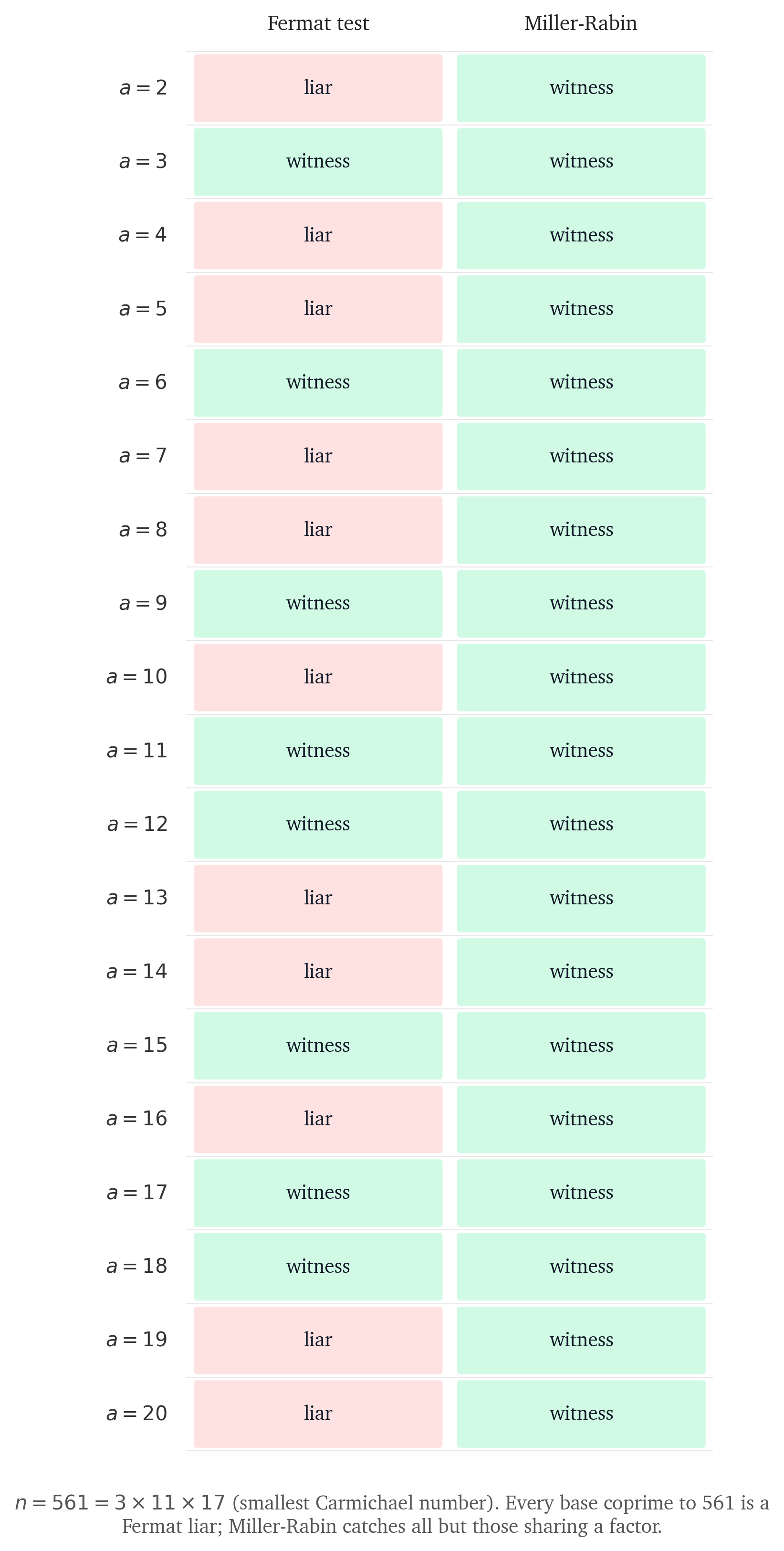
Is 561 prime? Trial division says no ($3 \times 11 \times 17$). But check $2^{560} \bmod 561$: you get 1, exactly what a prime would give. Try $5^{560} \bmod 561$: also 1. Try any base coprime to 561: always 1. Every test of this form says 561 is prime.

561 is the smallest number with this property. It fools not just one unlucky test, but every instance of the oldest and most natural primality test. It took 340 years of fixes to nearly close the gap.

# Background

Given an arbitrary integer $n$, how do you decide whether it’s prime?

The stakes are not abstract. RSA key generation requires finding two large primes $p$ and $q$, typically 1024 bits each, so that their product $n = pq$ is hard to factor. The security of RSA rests on the assumption that factoring $n$ is computationally infeasible, but that assumption is worthless if $p$ or $q$ is not actually prime. A composite that slips through primality testing produces a key that can be factored trivially. RSA, Diffie-Hellman, and most public-key cryptography depend on reliably generating large primes.

# Trial division

The oldest approach: to test whether $n$ is prime, try dividing it by every integer from 2 up to $\sqrt{n}$. If none divide evenly, $n$ is prime.

This works because if $n = ab$ with $a \le b$, then $a \le \sqrt{n}$. So we only need to check potential factors up to the square root. A standard optimization: after checking 2, only test odd divisors (or better, only test primes up to $\sqrt{n}$, but generating those primes is itself a sub-problem – the Sieve of Eratosthenes handles it for moderate bounds).

The complexity is $O(\sqrt{n})$ divisions. For a 10-digit number, that is roughly 100,000 divisions – fast on current hardware. For a 300-digit number (a typical RSA prime), $\sqrt{n}$ has 150 digits. There are approximately $10^{150}$ candidate divisors. At $10^{12}$ divisions per second, this would take about $10^{138}$ seconds. The universe is approximately $4 \times 10^{17}$ seconds old.

The issue is that $O(\sqrt{n})$ is exponential in the bit-length of $n$. If $n$ has $b$ bits, then $\sqrt{n} = 2^{b/2}$, and we need $2^{b/2}$ divisions. A polynomial-time algorithm would need $O(b^c)$ operations for some constant $c$. Trial division is correct and deterministic, but for cryptographic sizes it is useless. This is not a constant-factor problem that faster hardware will solve. The gap is exponential.

# The probabilistic trade

This gap (between what we need, testing 1024-bit numbers, and what deterministic methods can do in reasonable time) motivates a radical idea: accept a test that might be wrong.

A probabilistic primality test gives one of two answers: “definitely composite” or “probably prime.” In the language of randomized algorithms, this is a Monte Carlo algorithm: it always terminates in bounded time, but the answer might be wrong.The contrast is a Las Vegas algorithm, which always gives the correct answer but whose runtime is a random variable. ECPP (discussed below) is closer to the Las Vegas model: it always produces a correct certificate, but finding one can take unpredictable time. The naming is a gambling joke from the 1970s. The “probably” comes with a quantifiable error bound. If the probability of a false “probably prime” answer is less than $2^{-128}$, that is a smaller failure probability than a cosmic ray flipping a bit in your CPU during the computation. For engineering purposes, “probably prime with error $< 2^{-128}$” is as good as “proven prime.”

The challenge is building a test with: (1) an error probability that decreases exponentially with the number of iterations, and (2) no blind spots: no class of composites that always fools the test regardless of how many iterations you run.

The first condition is achievable: run the test multiple times with independent random choices, and error probabilities multiply (shrinking exponentially). The second took 340 years from Fermat to Rabin, because the natural first attempt, the Fermat test, has exactly the blind spot we need to avoid.

# Fermat’s Little Theorem

In 1640, Pierre de Fermat stated a theorem that would become foundational to primality testing:

$$a^{p-1} \equiv 1 \pmod{p}$$

for any prime $p$ and integer $a$ not divisible by $p$.

Consider the $p-1$ nonzero residues $\{1, 2, \ldots, p-1\}$ modulo $p$. Multiplying each by $a$ (with $\gcd(a, p) = 1$) permutes this set: the map $x \mapsto ax \bmod p$ is a bijection on $\{1, \ldots, p-1\}$. Therefore:

$$\prod_{i=1}^{p-1} (a \cdot i) \equiv \prod_{i=1}^{p-1} i \pmod{p}$$

The left side is $a^{p-1} \cdot (p-1)!$ and the right side is $(p-1)!$. Since $p$ is prime, $(p-1)!$ is invertible mod $p$, giving $a^{p-1} \equiv 1$.

The contrapositive gives us a primality test: if $a^{n-1} \not\equiv 1 \pmod{n}$ for some $a$ coprime to $n$, then $n$ is definitely composite.

# The Fermat Primality Test

This observation leads to a simple probabilistic test:

1. Pick a random base $a$ with $1 < a < n-1$
2. Compute $a^{n-1} \mod n$
3. If the result is not 1, $n$ is composite
4. If the result is 1, $n$ is probably prime

Step 2 uses modular exponentiation by repeated squaring, which runs in $O(\log n)$ multiplications mod $n$, each costing $O((\log n)^2)$ with schoolbook multiplication. Total: $O((\log n)^3)$. This scales with the number of digits, not the magnitude, which is exactly what we need.

Note an asymmetry: the test can prove compositeness (if $a^{n-1} \not\equiv 1$, $n$ is definitely composite) but can only suggest primality (if $a^{n-1} \equiv 1$, $n$ might be prime). This one-sided error structure defines probabilistic primality testing. We will never get a false “composite” answer, only a false “probably prime.”

The weakness: composite numbers that pass this test exist.

# Pseudoprimes

A composite number $n$ is called a Fermat pseudoprime to base $a$ if $a^{n-1} \equiv 1 \pmod{n}$.

For example, $341 = 11 \times 31$ is a pseudoprime to base 2:

$$2^{340} \equiv 1 \pmod{341}$$

Why does this happen? The order of 2 modulo 11 is 10 (by Fermat’s little theorem, $2^{10} \equiv 1 \pmod{11}$), and the order of 2 modulo 31 is 5 (since $2^5 = 32 \equiv 1 \pmod{31}$). Since $10 \mid 340$ and $5 \mid 340$, we get $2^{340} \equiv 1$ modulo both 11 and 31, hence modulo $341$ by the Chinese Remainder Theorem.

This means the Fermat test with base 2 incorrectly identifies 341 as “probably prime.”

The pseudoprimes to base 2 below 1000 are just 341 and 561. They are rare (there are only 245 base-2 pseudoprimes below $10^6$), but their rarity is deceptive. It might suggest that testing multiple bases would catch all composites: if $n$ is a pseudoprime to base 2, surely it fails for base 3? Often yes. 341 fails for base 3. But 561, as the opening promised, does not fail for any base.

# Carmichael Numbers

A composite number that is a pseudoprime to every base coprime to it is called a Carmichael number – and 561 is the smallest.15Vaclav Simerka found several examples in 1885, publishing in Casopis pro pestovani mathematiky a fysiky, a Czech-language journal with limited circulation outside Bohemia. His priority was recovered over a century later by Kral, Loebl, and Matousek (2001). In 1899, Alwin Korselt characterized them: a composite $n$ is a Carmichael number if and only if:

1. The number $n$ is square-free (no repeated prime factors)
2. For every prime $p$ dividing $n$, we have $(p-1) \mid (n-1)$

Korselt knew of no examples. In 1910, Robert D. Carmichael independently discovered 561. Why does it work? $561 - 1 = 560 = 2^4 \times 5 \times 7$, and:

• $3 - 1 = 2$ divides 560
• $11 - 1 = 10$ divides 560
• $17 - 1 = 16$ divides 560

The Fermat test fails completely on Carmichael numbers: no choice of base (coprime to $n$) will reveal their compositeness. For the Fermat test, Carmichael numbers are an unconditional blind spot. No amount of repetition helps.

Korselt’s criterion has an intuitive interpretation: it says that $n$ “pretends” to be prime by having its prime factors’ orders all divide $n - 1$. The Chinese Remainder Theorem then forces $a^{n-1} \equiv 1 \pmod{n}$ for all $a$ coprime to $n$. The deception is structural, not coincidental.

# How many exist?

For decades, mathematicians wondered whether there are infinitely many Carmichael numbers. In 1994, Alford, Granville, and Pomerance proved there are:6 for sufficiently large $x$, the number of Carmichael numbers up to $x$ exceeds $x^{2/7}$. The proof is non-constructive, and the $x^{2/7}$ figure is a lower bound on the proved lower bound, not an estimate of the true density. Harman (2005) pushed the proved lower bound to $x^{0.332}$, and Pinch’s exhaustive tabulation through $10^{21}$ shows the empirical count growing closer to $x^{0.35}$ – still far below Erdos’s conjecture that the count up to $x$ is $x^{1-o(1)}$, which remains open.

# Solovay-Strassen: The First Probabilistic Test

Carmichael numbers force a choice: either find a completely different kind of test, or accept that the Fermat test has an unconditional blind spot. In 1977, Robert Solovay and Volker Strassen found the first option.1 Their insight: check not just whether $a^{n-1} \equiv 1$, but whether the path to 1 is consistent with primality. The tool is the Euler criterion, which connects modular exponentiation to the Legendre symbol.

Lemma (Euler criterion). For an odd prime $p$ and $\gcd(a, p) = 1$:

$$a^{(p-1)/2} \equiv \left(\frac{a}{p}\right) \pmod{p}$$

where $\left(\frac{a}{p}\right)$ is the Legendre symbol ($+1$ if $a$ is a quadratic residue mod $p$, $-1$ otherwise).

Proof sketch. Since $\mathbb{F}_p^\times$ is cyclic of order $p-1$, we have $a^{p-1} \equiv 1$, so $a^{(p-1)/2}$ is a square root of 1, hence $\pm 1$. Write $a = g^j$ for a generator $g$. Then $a^{(p-1)/2} = g^{j(p-1)/2}$. When $j$ is even, this is $(g^{p-1})^{j/2} = 1$, so $a$ is a quadratic residue. When $j$ is odd, $g^{j(p-1)/2} = g^{(p-1)/2} = -1$ (the unique element of order 2), so $a$ is a non-residue.

The Solovay-Strassen test: pick a random $a$, compute both $a^{(n-1)/2} \bmod n$ and the Jacobi symbol $\left(\frac{a}{n}\right)$ (which can be computed in $O(\log^2 n)$ by reciprocity, without knowing the factorization of $n$). If they disagree, $n$ is composite.

Why this breaks the Carmichael barrier: a Carmichael number $n$ satisfies $a^{n-1} \equiv 1 \pmod{n}$ for all $a$ coprime to $n$, but this does not force $a^{(n-1)/2} \equiv \left(\frac{a}{n}\right)$. The Jacobi symbol factors multiplicatively over the prime factors of $n$, while the power $a^{(n-1)/2}$ does not decompose the same way. Solovay and Strassen proved that for any composite $n$, at least half of all bases $a$ in $\{1, \ldots, n-1\}$ are witnesses – the Euler criterion fails for them. This gives a $1/2$ error bound per round, worse than Miller-Rabin’s $1/4$ but sufficient to bypass Carmichael numbers entirely.

# Why Primes Are Algebraically Special

The Fermat test checks one property of primes: $a^{p-1} \equiv 1$. Miller’s test checks a deeper property: not just what the final value is, but how it got there. Fermat asks “is the answer 1?” Miller asks “what is the square root of that 1?” In a prime field, the only square roots of 1 are $\pm 1$. In a composite ring, there are others, and finding one proves compositeness. To understand why, we need a fact about the multiplicative group modulo a prime.

When $p$ is prime, $\mathbb{F}_p^\times = \{1, 2, \ldots, p-1\}$ under multiplication is a cyclic group of order $p-1$. Every element is a power of some generator $g$. A consequence: the equation $x^2 \equiv 1 \pmod{p}$ has exactly two solutions: $x = 1$ and $x = -1$. This is because $x^2 - 1 = (x-1)(x+1)$, and in a field, each factor has at most one root.

For composite $n$, $(\mathbb{Z}/n\mathbb{Z})^\times$ is not cyclic in general – by the Chinese Remainder Theorem, it decomposes as a product of the groups for each prime factor. This product structure creates extra square roots of unity: elements $x$ with $x^2 \equiv 1 \pmod{n}$ but $x \not\equiv \pm 1 \pmod{n}$. For example, $4^2 = 16 \equiv 1 \pmod{15}$, but $4 \not\equiv \pm 1$.

These non-trivial square roots cannot exist modulo a prime but do exist modulo composites. Miller’s test detects them.

# Strong Pseudoprimes and Miller’s Test

In 1976, Gary Miller observed that we can strengthen the Fermat test by exploiting the algebraic structure above.2

Write $n - 1 = 2^s \cdot d$ where $d$ is odd. For a prime $p$ and base $a$ coprime to $p$, one of the following must hold:

$$a^d \equiv 1 \pmod{p}$$

or

$$a^{2^r d} \equiv -1 \pmod{p} \quad \text{for some } 0 \le r < s$$

Why must one of these hold? Start from Fermat: $a^{p-1} = a^{2^s d} \equiv 1 \pmod{p}$. Now consider the squaring chain:

$$a^d, \; a^{2d}, \; a^{4d}, \; \ldots, \; a^{2^s d}$$

The last term is 1. Each term is the square of the previous. Working backwards from $a^{2^s d} \equiv 1$: if $a^{2^r d} \equiv 1$, then $a^{2^{r-1} d}$ is a square root of 1 modulo $p$. In a field (which $\mathbb{Z}/p\mathbb{Z}$ is, since $p$ is prime), the polynomial $x^2 - 1$ has at most two roots: $+1$ and $-1$. So either the previous term is also 1 (and we continue backwards) or it is $-1$ (and we stop). Eventually we either reach $a^d \equiv 1$ or find some $a^{2^r d} \equiv -1$.

The critical point: for a composite $n$, $\mathbb{Z}/n\mathbb{Z}$ is not a field, and $x^2 \equiv 1 \pmod{n}$ can have more than two solutions. For example, modulo $n = 15$, we have $4^2 = 16 \equiv 1$ – a “non-trivial square root of unity.” This is the crack that Miller’s test exploits.

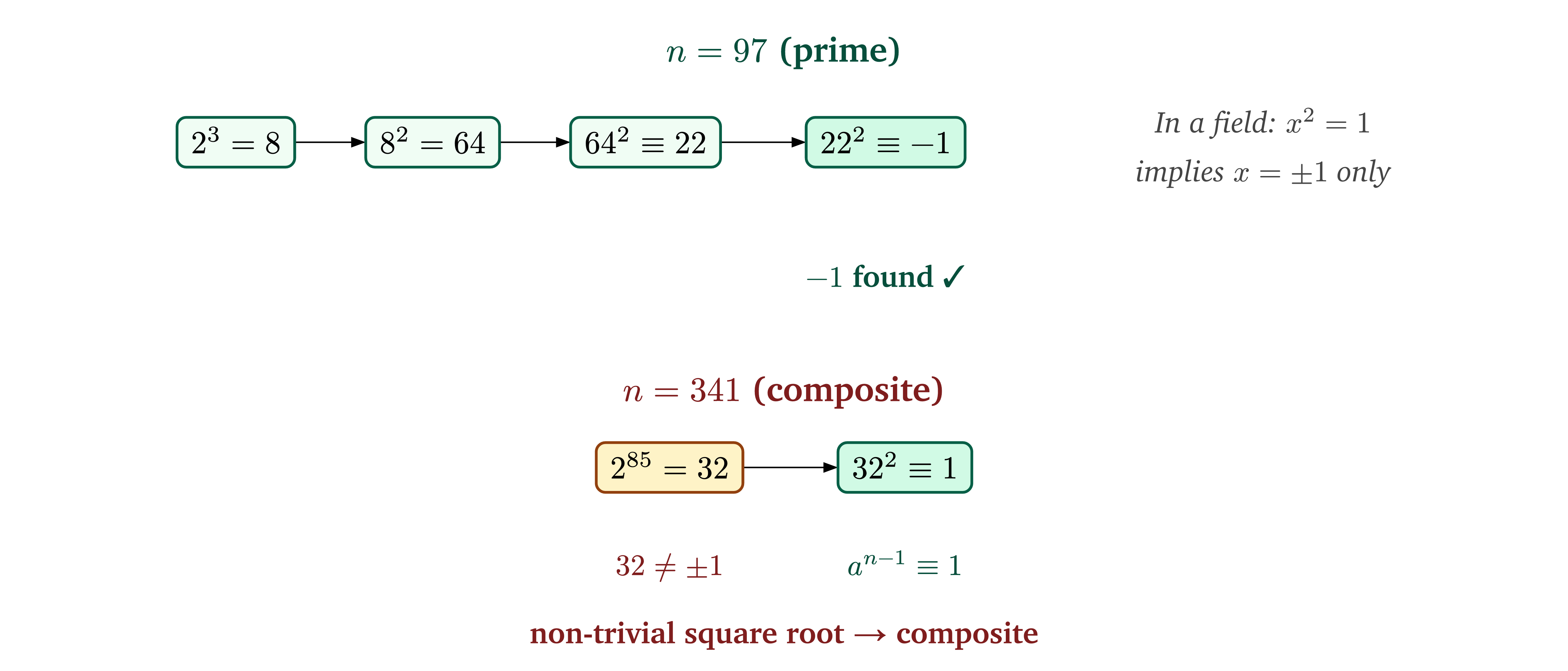
Worked example: $n = 341$, $a = 2$. Recall that 341 passes the Fermat test for base 2. Write $341 - 1 = 340 = 2^2 \times 85$, so $s = 2$ and $d = 85$. The squaring chain is:

$$2^{85} \bmod 341 = 32, \quad 32^2 \bmod 341 = 1024 \bmod 341 = 1$$

The chain went from 32 to 1 in one squaring. But $32 \not\equiv 1$ and $32 \not\equiv -1 \pmod{341}$ (since $-1 \equiv 340$). So 32 is a non-trivial square root of 1 modulo 341 – exactly the kind of witness that cannot exist modulo a prime. Miller’s test correctly identifies 341 as composite. The Fermat test missed this because it only checks the final value $2^{340} \bmod 341 = 1$, discarding the information in the intermediate steps.

A composite number that passes this stronger test for base $a$ is called a strong pseudoprime to base $a$. Unlike the Fermat test, there are no “strong Carmichael numbers”: no composite passes for all bases.

# The Miller-Rabin Test

In 1980, Michael Rabin made Miller’s test probabilistic and proved a key result:3 for any composite $n$, at most $1/4$ of bases $a$ in $\{2, \ldots, n-2\}$ are strong liars (bases for which $n$ passes the strong test). Louis Monier independently proved the same bound the same year.

Theorem (Rabin and Monier, 1980).3 If $n$ is an odd composite, the number of strong liars in $\{1, \ldots, n-1\}$ is at most $\frac{n-1}{4}$.

Proof sketch. Write $n - 1 = 2^s d$ with $d$ odd. By the Chinese Remainder Theorem, $(\mathbb{Z}/n\mathbb{Z})^\times \cong \prod_{i} (\mathbb{Z}/p_i^{e_i}\mathbb{Z})^\times$. A strong liar $a$ must have its squaring chain “look prime” – either $a^d \equiv 1$ or $a^{2^r d} \equiv -1$ for some $r$.

The key constraint: $a^{2^r d} \equiv -1 \pmod{n}$ requires $a^{2^r d} \equiv -1$ modulo every prime power factor simultaneously. But each factor has its own 2-adic structure ($p_i - 1 = 2^{s_i} d_i$ with possibly different $s_i$), so the squaring chains must “synchronize” across all factors at the same step $r$. The strong liars form a subgroup of $(\mathbb{Z}/n\mathbb{Z})^\times$. The synchronization constraint forces this subgroup to have index at least 4.

The worst case is $n = pq$ with $p \equiv q \equiv 3 \pmod{4}$ and $\gcd(p-1, q-1) = 2$, which gives exactly $\frac{n-1}{4}$ strong liars. All other composites have fewer.

This means:

• Each iteration has at most $1/4$ probability of being fooled
• After $k$ iterations with independent random bases, the error probability is at most $(1/4)^k$
• With 40 iterations, the error probability is less than $10^{-24}$

But most composites are caught by the first random base. Damgard, Landrock, and Pomerance11 showed that for random odd $k$-bit composites, the average-case error probability after $t$ rounds drops as $\exp(-c\sqrt{kt})$ for a constant $c$, much faster than the worst-case $4^{-t}$. For 1024-bit numbers with even a single round, the average-case error probability is negligible.

Unlike the Fermat test, Miller-Rabin is not fooled by Carmichael numbers. For any Carmichael number $n$, at least 75% of bases reveal its compositeness through the strong pseudoprime check. The “non-trivial square roots of unity” that exist in $\mathbb{Z}/n\mathbb{Z}$ (but not in $\mathbb{Z}/p\mathbb{Z}$) always provide witnesses.

# Implementation

Modular exponentiation by repeated squaring makes each round efficient. Here is a complete Miller-Rabin test in Python:

import random

def is_probable_prime(n, k=40):
    """Miller-Rabin with k rounds. False = composite, True = probably prime."""
    if n < 2: return False
    if n < 4: return True
    if n % 2 == 0: return False
    # Write n - 1 = 2^s * d with d odd
    d, s = n - 1, 0
    while d % 2 == 0:
        d //= 2
        s += 1
    for _ in range(k):
        a = random.randrange(2, n - 1)
        x = pow(a, d, n)          # a^d mod n
        if x == 1 or x == n - 1:
            continue
        for _ in range(s - 1):
            x = pow(x, 2, n)      # square mod n
            if x == n - 1:
                break
        else:
            return False           # composite witness found
    return True

Python’s built-in three-argument pow(a, d, n) performs modular exponentiation by repeated squaring internally; it does not compute $a^d$ and then reduce. This makes the implementation efficient even for thousand-bit inputs. With $k = 40$ rounds, the error probability is below $4^{-40} \approx 10^{-24}$, which is the typical choice for cryptographic key generation.

The for/else construct is Python-specific: the else clause executes only if the inner for loop completes without break, meaning none of the squarings produced $-1$, so $a$ is a witness to compositeness.

# Deterministic Variants

# Miller’s test under GRH

Miller’s original 1976 test was not probabilistic; it was deterministic, conditional on the extended Riemann hypothesis (ERH). Under ERH, Miller proved that for any composite $n$, there exists a witness $a < 2 (\ln n)^2$. This means you only need to test bases up to $O((\log n)^2)$, giving a deterministic polynomial-time test – if ERH is true.

ERH remains unproven. The conditional result ties the difficulty of deterministic primality testing to the distribution of zeros of the Riemann zeta function.

# Known deterministic witness sets

Even without ERH, exhaustive computation has established that specific small sets of bases suffice for bounded ranges. These results turn Miller-Rabin into a deterministic test for numbers below each bound:

The last bound is approximately $3.3 \times 10^{24}$. For 64-bit integers ($< 2^{64} \approx 1.8 \times 10^{19}$), the first 12 primes as bases give a deterministic test. Alternatively, Jim Sinclair’s 7-element non-prime set $\{2, 325, 9375, 28178, 450775, 9780504, 1795265022\}$ is sufficient for the same range with one fewer test; this is what production implementations such as Rust’s num-prime and Go’s math/big use. This is how many implementations handle “small” numbers: no randomness needed, no probability of error, and the test runs in microseconds.

The smallest strong pseudoprime to base 2 is 2047 – which is why base $\{2\}$ alone suffices below that threshold.

# BPSW: the pragmatic gold standard

Miller-Rabin with random bases has no blind spots – but each round is probabilistic, and 40 rounds is slow for bulk prime generation. Can we do better with fewer tests by choosing them to be complementary? The Baillie-PSW test, introduced in 1980 by Robert Baillie,4 Carl Pomerance, John Selfridge, and Samuel Wagstaff,5 combines two tests that fail on disjoint sets of composites:

1. A Miller-Rabin test to base 2
2. A strong Lucas probable prime test (with a specific parameter selection method)

A composite that slips through Miller-Rabin base 2 typically fails the Lucas test. The power of BPSW comes from the near-disjointness of the two pseudoprime sets: the number-theoretic properties that make a number a strong pseudoprime (multiplicative order structure in $(\mathbb{Z}/n\mathbb{Z})^\times$) are largely independent of those that make it a Lucas pseudoprime (quadratic residue structure in a degree-2 extension). For a composite to fool both tests simultaneously, it would need to “look prime” in two algebraically unrelated ways – and no such number has ever been found.

The Lucas test works in a different algebraic setting. Given parameters $P$ and $Q$ with discriminant $D = P^2 - 4Q$, define the Lucas sequences $U_k(P,Q)$ and $V_k(P,Q)$ via the recurrence $U_{k+1} = PU_k - QU_{k-1}$. For a prime $p$ with Jacobi symbol $(D/p) = -1$, we have $U_{p+1} \equiv 0 \pmod{p}$. The “strong” variant adds a squaring chain similar to Miller-Rabin. The parameter selection (Selfridge’s Method A: choose the first $D$ in the sequence $5, -7, 9, -11, \ldots$ such that $(D/n) = -1$) is designed to maximize the independence between the Miller-Rabin and Lucas tests. The strong Lucas test has its own standalone error bound: Einsele and Paterson (2024) proved the strong liar fraction is at most $4/15$, slightly worse than Miller-Rabin’s $1/4$ in isolation. A strong Lucas evaluation costs roughly 2–3× a single Miller-Rabin round, so BPSW’s two-test structure is not free, but the complementarity makes it far more effective than running two Miller-Rabin rounds.

No BPSW counterexample has ever been found. The original 1980 paper offered a $30 reward for a counterexample (from Pomerance, Selfridge, and Wagstaff).5 In 2021, Baillie, Fiori, and Wagstaff14 offered $2,000 for a counterexample to a strengthened variant. Neither reward has been claimed. Exhaustive search has verified that no counterexample exists below $2^{64}$.

BPSW requires only two tests (one modular exponentiation + one Lucas computation), making it faster than running 40 rounds of Miller-Rabin. It is the default primality test in many implementations, including Mathematica, Maple, and SageMath.

# Beyond Miller-Rabin

Miller-Rabin and BPSW are probabilistic (or deterministic only for bounded ranges). For some applications (primality certificates, mathematical proofs, record-keeping) we need tests that prove primality unconditionally.

# AKS: theoretical breakthrough

In 2002, Manindra Agrawal, Neeraj Kayal, and Nitin Saxena proved that primality is in P:7The preprint circulated in August 2002. The journal publication in Annals of Mathematics appeared in 2004. Dates in citations refer to journal publication; “2002” in prose refers to when the result became known. there exists a deterministic polynomial-time algorithm that decides primality without any unproven hypothesis. AKS was the first test that is simultaneously general (works for all integers), polynomial-time, deterministic, and unconditionally correct. Every previous test satisfied at most three of these four properties: trial division is general, deterministic, and correct but exponential; Miller-Rabin is general, polynomial, and (conditionally) correct but either probabilistic or conditional on ERH; ECPP is general and polynomial but heuristic in its runtime analysis.

Kayal and Saxena were BTech students of Agrawal at IIT Kanpur. The preprint circulated in August 2002 and triggered an immediate burst of activity; Berrizbeitia, Lenstra-Pomerance, and Bernstein all submitted variants within weeks, rapidly tightening the complexity from the original $\tilde{O}((\log n)^{12})$.

The original algorithm runs in $\tilde{O}((\log n)^{12})$ time. Lenstra and Pomerance8 improved this to $\tilde{O}((\log n)^6)$ in 2005. The key idea starts from a classical observation: if $n$ is prime, then the polynomial identity

$$(x + a)^n \equiv x^n + a \pmod{n}$$

holds in $\mathbb{Z}_n[x]$ for all $a$ (this is essentially the Frobenius endomorphism). For composite $n$, this identity generally fails. But checking it directly requires working with a polynomial of degree $n$ – which is as expensive as trial division.

AKS’s insight is to check this identity modulo a polynomial $x^r - 1$ for a suitable small $r$: verify $(x + a)^n \equiv x^{n \bmod r} + a$ in $\mathbb{Z}_n[x]/(x^r - 1)$. Now the polynomials have degree at most $r$, and $r$ can be chosen as $O((\log n)^5)$ or better.

The key lemma: if $(x + a)^n \equiv x^n + a \pmod{n, x^r - 1}$ holds for $a = 1, 2, \ldots, \lfloor\sqrt{\phi(r)} \log n\rfloor$, and $n$ has no prime factor $\le r$, and $n$ is not a perfect power, then $n$ is prime. The proof constructs a group $G$ of residues in $(\mathbb{Z}/n\mathbb{Z})[x]/(x^r - 1)$ generated by $\{x + 1, x + 2, \ldots\}$ and shows that $|G|$ is both large (from the many verified identities) and small (from the structure of the quotient ring), forcing $n$ to be prime. The total number of checks is polynomial in $\log n$.

AKS is not used in practice. For 64-bit numbers, BPSW is orders of magnitude faster. For larger numbers, ECPP (below) is faster and also produces a certificate. AKS is a “galactic algorithm”: polynomial in theory, but with constants so large that Miller-Rabin with 64 rounds is faster by orders of magnitude even for 1024-bit inputs. Its significance is theoretical, settling a long-standing complexity question, not providing a practical tool.A galactic algorithm is one that is asymptotically optimal but whose constant factors are so large that it is never faster than simpler methods on any input that fits in the observable universe.

# ECPP: the practical gold standard for proven primes

Elliptic Curve Primality Proving (ECPP) was developed by Shafi Goldwasser and Joe Kilian in 1986,10 and refined into a practical algorithm by A. O. L. Atkin and Francois Morain in 1993.9 It runs in $\tilde{O}((\log n)^5)$ heuristic time and produces a primality certificate – a compact proof that anyone can verify much faster than it took to produce.

The core idea uses elliptic curves over $\mathbb{Z}/n\mathbb{Z}$. Given a point $P$ on an elliptic curve $E$ modulo $n$, if we can show that the group order $|E(\mathbb{Z}/n\mathbb{Z})|$ has a large prime factor $q$, and certain conditions hold, then either $n$ is prime or $n$ has a very small factor (which we can check by trial division). The problem then reduces to proving $q$ is prime, a smaller instance of the same problem. This recursive structure terminates quickly.

The certificate is an Atkin-Goldwasser-Kilian-Morain certificate: a chain of elliptic curves and points that witnesses primality at each recursive step. Verification runs in polynomial time and does not require trusting the prover’s computation. This is the key distinction from probabilistic tests: ECPP does not say “probably prime with high confidence.” It says “here is a proof; check it yourself.” The certificate for a 10,000-digit prime might be a few megabytes, but verifying it takes minutes rather than the hours needed to produce it.

ECPP holds the record for the largest proven prime with a general-purpose algorithm: $R(109297) = (10^{109297} - 1)/9$, a repunit with 109,297 digits. (Mersenne primes are tested with the deterministic Lucas-Lehmer test, which exploits their special form.)

# Comparison

Each successive test in this post exploits more algebraic structure of finite fields. The Fermat test checks multiplicative group order. Miller-Rabin probes the 2-Sylow subgroup via the squaring chain.The 2-Sylow subgroup is the largest subgroup whose order is a power of 2 – it’s what the squaring chain decomposes. When $n - 1 = 2^s d$, the chain $a^d, a^{2d}, \ldots, a^{2^s d}$ walks through this subgroup. The Lucas test probes quadratic extensions $\mathbb{F}_{p^2}$. ECPP uses the group structure of elliptic curves over $\mathbb{F}_p$.

# How Real Systems Test Primality

Real systems do not just run Miller-Rabin in a loop. The full pipeline for generating an RSA prime in OpenSSL (as of version 3.x) looks like this:

1. Generate a random odd number $n$ of the desired bit length, with the top two bits set (to ensure the product $pq$ has the right bit length).
2. Check divisibility by a table of small primes (typically the first 2048 primes). This is trial division with a fixed bound, and it rejects about 80% of candidates cheaply.
3. Run one round of Miller-Rabin with base 2.
4. Run a Lucas test (the second half of BPSW).
5. Depending on the security level and standard being followed, run additional Miller-Rabin rounds with random bases.

GMP’s mpz_probab_prime_p function follows a similar structure: trial division, then BPSW, then optional additional Miller-Rabin rounds requested by the caller.

The FIPS 186-5 standard (the current revision for US government systems) specifies Miller-Rabin with iteration counts that depend on the required error probability and the bit length of the candidate. For 1024-bit primes (half of a 2048-bit RSA modulus), FIPS 186-5 Appendix C.1 requires only 4 Miller-Rabin rounds to achieve the target error probability – far fewer than the generic 40-round recommendation – because the average-case error for near-random large primes drops dramatically faster than the $4^{-t}$ worst-case bound.

libsodium, used widely for NaCl-family cryptography, relies on Ed25519 (which uses a fixed curve, not generated primes) for signatures, so primality testing is not in its hot path. But for applications that do need prime generation, libsodium defers to the OS or to a constant-time Miller-Rabin implementation.

The primality test itself is rarely the bottleneck. For a 2048-bit RSA modulus, the expected number of random candidates before finding a prime is approximately $\ln(2^{1024}) \approx 710$ (by the prime number theorem). Each candidate undergoes trial division first, which filters out most composites in microseconds. Only the ~20% that survive trial division reach the expensive probabilistic test. End-to-end, generating both primes typically takes a few hundred milliseconds.

# Timing side channels

Every step in this pipeline must run in constant time. If the Miller-Rabin test takes longer for primes than for composites, an attacker observing timing can learn which candidates were selected as primes, narrowing the search space for factoring $n = pq$.

The attack surface is concrete. In the squaring chain, a composite is detected as soon as a witness is found; if the implementation returns early, the execution time leaks whether $n$ passed or failed. A prime survives all $s$ squaring steps; a composite caught at step $r < s$ returns faster. The timing difference is small (microseconds), but it is measurable across many key generation attempts, and it is enough to bias an attacker’s factoring search.

Production implementations defend with two techniques. First, Montgomery multiplication: all modular arithmetic uses Montgomery form, which replaces division by $n$ (whose cost depends on the value of $n$) with a fixed sequence of multiplications and bit shifts, making the cost of each operation independent of the operands’ values. Second, fixed iteration counts: the squaring loop always executes all $s$ steps regardless of whether a witness appeared at step $r < s$. The result is the same number of multiplications for primes and composites.

A timing-leaky primality test is a broken primality test for cryptographic purposes, even if its mathematical properties are perfect.13

# Open Problems

# The BPSW question

The central open problem in practical primality testing: does a BPSW counterexample exist?

Heuristic arguments suggest counterexamples should exist but be astronomically rare. Pomerance has estimated12 that if they exist, the smallest might exceed $10^{10000}$. Exhaustive search has checked all numbers below $2^{64}$ with no counterexample found.

The $2,000 bounty (Baillie-Fiori-Wagstaff14) remains unclaimed. If no counterexample exists, proving this would likely require new techniques in analytic number theory. If one exists, finding it would likely require new techniques in constructive algebra.

Either resolution would be significant. In the meantime, BPSW occupies a peculiar status: universally trusted in practice, with no theoretical proof of correctness, and with heuristic arguments that counterexamples should exist but haven’t been found.

# References

[1] Solovay, R. & Strassen, V. (1977). “A Fast Monte-Carlo Test for Primality.” SIAM Journal on Computing, 6(1), 84-85. ↩

[2] Miller, G. L. (1976). “Riemann’s Hypothesis and Tests for Primality.” Journal of Computer and System Sciences, 13(3), 300-317. ↩

[3] Rabin, M. O. (1980). “Probabilistic Algorithm for Testing Primality.” Journal of Number Theory, 12(1), 128-138. ↩

[4] Baillie, R. & Wagstaff, S. S. (1980). “Lucas Pseudoprimes.” Mathematics of Computation, 35(152), 1391-1417. ↩

[5] Pomerance, C., Selfridge, J. L. & Wagstaff, S. S. (1980). “The Pseudoprimes to 25 x 10^9.” Mathematics of Computation, 35(151), 1003-1026. ↩

[6] Alford, W. R., Granville, A. & Pomerance, C. (1994). “There Are Infinitely Many Carmichael Numbers.” Annals of Mathematics, 139(3), 703-722. ↩

[7] Agrawal, M., Kayal, N. & Saxena, N. (2004). “PRIMES Is in P.” Annals of Mathematics, 160(2), 781-793. ↩

[8] Lenstra, H. W. & Pomerance, C. (2019). “Primality Testing with Gaussian Periods.” Journal of the European Mathematical Society, 21(4), 1229–1269. (Manuscript circulated 2005.) ↩

[9] Atkin, A. O. L. & Morain, F. (1993). “Elliptic Curves and Primality Proving.” Mathematics of Computation, 61(203), 29-68. ↩

[10] Goldwasser, S. & Kilian, J. (1986). “Almost All Primes Can Be Quickly Certified.” Proceedings of the 18th STOC, 316-329. ↩

[11] Damgard, I., Landrock, P. & Pomerance, C. (1993). “Average Case Error Estimates for the Strong Probable Prime Test.” Mathematics of Computation, 61(203), 177-194. ↩

[12] Pomerance, C. (1981). “On the Distribution of Pseudoprimes.” Mathematics of Computation, 37(156), 587-593. ↩

[13] Crandall, R. & Pomerance, C. (2005). Prime Numbers: A Computational Perspective. 2nd ed. Springer. ↩

[14] Baillie, R., Fiori, A. & Wagstaff, S. S. (2021). “Strengthening the Baillie-PSW Primality Test.” Mathematics of Computation, 90(330), 1931-1955. ↩

[15] Kral, D., Loebl, M. & Matousek, J. (2001). “Simerka as a predecessor of Carmichael.” Expositiones Mathematicae, 19(4), 377–381. ↩