Sampling a biased coin with a fair coin
August 15, 2015revised September 20, 2026
Write a desired probability in binary, flip a fair coin until the first heads, and return the digit at that position. This produces the specified probability using two flips on average, or fewer when we recognize that the remaining digits are all zero.
How would you use a fair coin to choose something with probability ?
Flip until the first heads. If it arrives on an even-numbered flip, choose
the thing. Otherwise, don’t. The successful sequences are TH, TTTH,
TTTTTH, and so on, so their probabilities add up to
There is no rejection and restart. Every terminating run supplies an answer, including a heads on the first flip. The chance of still flipping after tosses is .
# Let the binary digits choose the outcome
Write the desired probability as
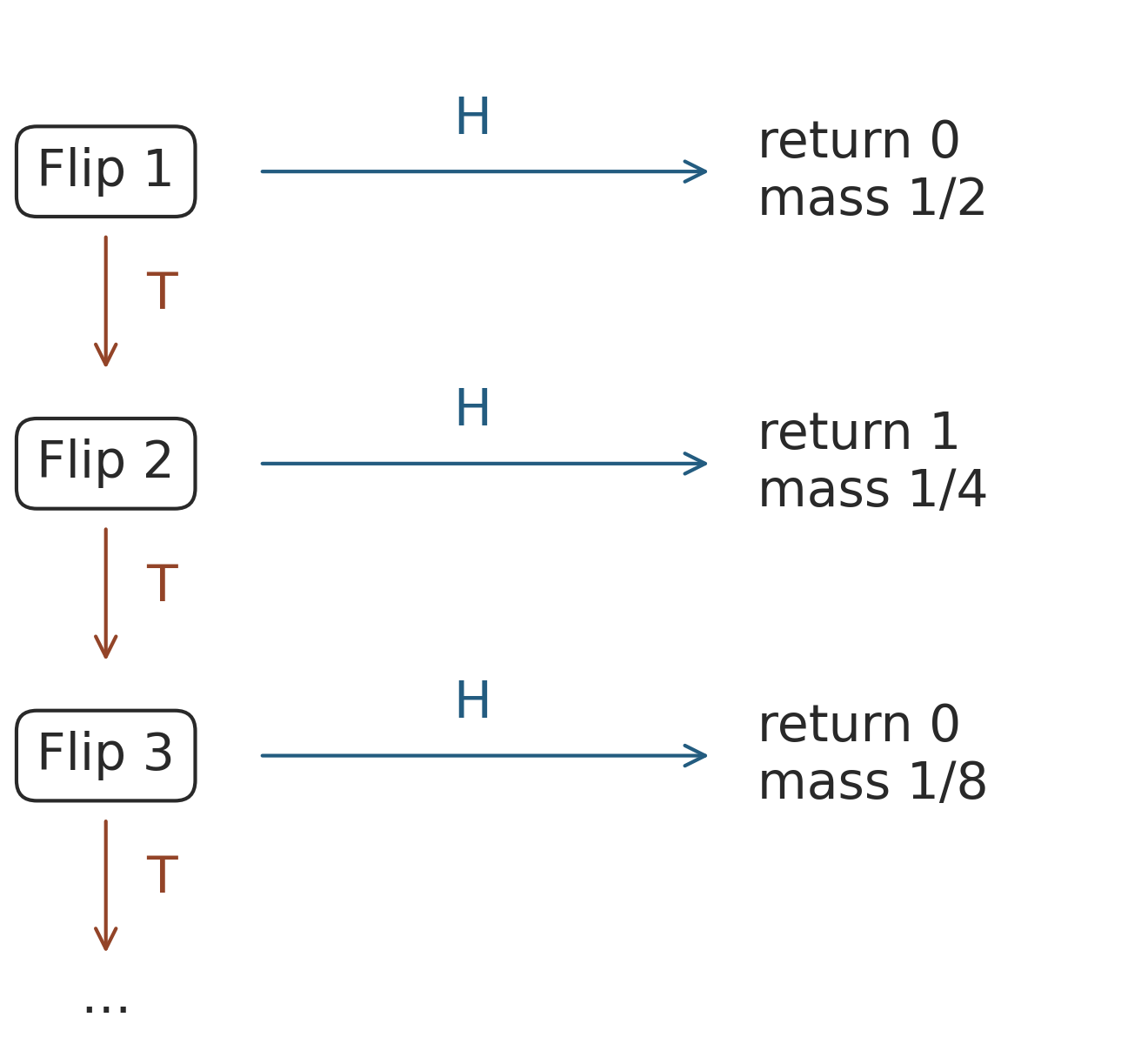
Flip a fair coin until the first heads. If that happens on flip , return . A returned 1 means success; a returned 0 means failure. This is a Bernoulli trial with parameter .
The first heads occurs at position with probability , so
The construction assigns the probability mass to the first digit, to the second, to the third, and so on. Those are exactly the place values in the binary expansion. For , the even-numbered digits are 1.
Reproduce this figure
tar -xf coin-sampling-gen_figures.tar && cd coin-sampling-gen_figures/coin-sampling && uv run --locked gen_figures.pyRequires uv and Python 3.12; the locked packages download on first run.
Lumbroso gives this geometric-index construction and an exact rational implementation in Appendix B of his paper on random-bit generation. It is an established sampling method, rather than a special property of one third.1
# Two flips on average, but no fixed limit
For any nonnegative integer-valued running time, its expectation is the sum of its tail probabilities. Each run of length contributes one to the first terms of that sum. Here this gives
This counts fair flips. Computing a requested digit of is separate work. For rational probabilities the digit calculation is a short integer operation; an arbitrary real number is not automatically an executable input.
The algorithm terminates with probability one. That does not give a fixed maximum runtime: after 20 flips the chance of still waiting is , about one in a million.
That distinction is unavoidable for . Any algorithm that always finishes within fair flips can be described using equally likely bit strings. Pad shorter runs with ignored flips. Its success probability must then be an integer multiple of , which cannot equal .
# When fewer flips suffice
A probability with a terminating binary expansion is called dyadic. For example,
The first-heads procedure returns 0 on H, and 1 on TH or TTH.
After TTT, every remaining digit is zero. There is no reason to keep
flipping: return 0 immediately. The four leaves have masses
, , , and ; the two success leaves sum to .
If is in lowest terms and , this modification has cost
| Desired probability | Expected fair flips | Maximum flips |
|---|---|---|
| or | ||
| Unbounded | ||
| Unbounded |
Use the terminating expansion for a dyadic number. Although , recognizing a constant tail is what allows the algorithm to finish without waiting for another heads.
# Why this cost is optimal
Imagine any exact algorithm as a binary tree: internal nodes request a fair flip, and leaves return 0 or 1. After flips, a path still in progress carries probability .
If is not dyadic, there must be an unfinished path at every finite depth. Otherwise, the algorithm would have the finite flip limit ruled out above. Consequently every exact sampler has
The digit construction attains equality at every depth. For a reduced dyadic , the same argument applies up to depth , and the modified construction again attains every bound.
This is optimality for one exact sample starting with no saved randomness, using independent fair bits as the sole random source. It says nothing by itself about processor time or the cost of a batch of samples. Knuth and Yao’s discrete distribution generating trees extend this reasoning to any finite collection of outcomes; Saad and colleagues state their binary-digit characterization in Theorem 2.1. 2
Lumbroso’s Appendix B concludes that the optimal cost is two for every Bernoulli parameter. The dyadic exception matters: the derivation uses , which fails when is an integer. Here the braces mean fractional part, and becomes an integer once a dyadic expansion terminates. The general tree result includes this exception.
# Exact arithmetic for rational probabilities
For , generate the binary digits by doubling the numerator. The quotient is the next digit; the remainder is the numerator for the next step. For , the remainders alternate between 2 and 1, producing digits 0 and 1 forever. Only the digits reached by the coin flips need to be computed.
def bernoulli(a, b, flip):
    """Return 1 with probability a/b; flip supplies independent fair bits."""
    if b <= 0 or not 0 <= a <= b:
        raise ValueError("require b > 0 and 0 <= a <= b")
    if a == b:
        return 1
    while a:
        digit, a = divmod(2 * a, b)
        if flip() == 1:
            return digit
    return 0
The inputs a and b are integers; flip() returns 0 or 1. The loop
keeps the remainder below b, so its integer storage is proportional to
, even when the expansion repeats forever. Python’s integers
avoid overflow in 2 * a; a fixed-width implementation must leave room
for that doubling.
The terminating condition is important. Returning the current digit before its coin flip when the remainder becomes zero would be wrong: for , it would always return 1. We must still distinguish the heads leaf from the tails branch.
For a simulation, a call might look like this:
import random

rng = random.Random(20150815)
result = bernoulli(1, 3, lambda: rng.getrandbits(1))
This is a reproducible pseudorandom simulation. The probability proof assumes independent fair bits. Also, requesting one bit from a generator does not necessarily consume only one bit of its internal output: efficient implementations can buffer a word and consume its bits across calls. Neither the proof nor this Python example establishes a speed advantage.
# What a floating-point comparison changes
The familiar random.random() < p uses a finite grid. Python’s
random() supplies 53 bits of precision, with possible values
for .
For a threshold , comparison against that grid accepts with
probability , assuming equiprobable grid
points. An intended decimal or fraction may also have been rounded when
converted to the floating-point threshold.
3
The discrepancy is tiny for many simulations. It is still a different contract from exact , and the distinction becomes visible for very small probabilities: any positive threshold below accepts the grid point zero, yielding probability .
Passing (1, 3) to the integer algorithm preserves the fraction. Passing
the exact integer ratio of a stored float instead preserves that float’s
dyadic value. Neither representation reconstructs an intended real number
that was already rounded away.
# Weighted choices
Suppose three outcomes have probabilities , , and . First accept A with probability . If that fails, choose B with conditional probability
If B also fails, choose C. The unconditional probabilities are
For nonnegative integer weights, no floating-point normalization is needed:
remaining = sum(weights)
for i, weight in enumerate(weights):
    if bernoulli(weight, remaining, flip):
        return i
    remaining -= weight
Require a nonempty list with at least one positive weight. Zero weights are skipped without using a flip; the last positive weight is selected with certainty if reached. In probability notation the $k$th trial uses , the probability remaining after all previous failures.
This extension is exact, but sequential choices are not generally optimal
in bits. Ordering matters. Four equal categories cost
flips on average under this procedure. Assigning
the four outcomes to 00, 01, 10, and 11 uses exactly two.
# An irrational probability without its digits
There is another way to build exact probabilities: compose simpler coins. For example, we can make a coin with success probability without calculating , taking a logarithm, or reading its binary expansion.
Imagine an initial success that costs no flip. Then try independent coins with success probabilities , , , and so on. Stop at the first failure. Return 1 if the total number of successes, including the initial one, is even.
def inverse_e(flip):
    n = 2
    while bernoulli(1, n, flip):
        n += 1
    return int((n - 1) % 2 == 0)
If is that success count, reaching at least successes has probability
For , the empty product is one. Therefore , and the probability of an even count is
The series also explains why the process terminates: its continuation probability decreases factorially. With our rational sampler, the expected number of fair flips is
where is the cost of the coin: two unless is a power of two, in which case the finite-tail saving applies. This is more than the two-flip digit sampler would use for , but the only probabilities we need to represent are integer fractions.
Flajolet, Pelletier, and Soria study this broader idea under the name Buffon machines: finite procedures driven by fair coins that produce specified probabilities, including irrational ones. Their paper develops exponential-probability generators in Section 2.2. The rational-coin parity construction above is a composition whose proof is given here, rather than a transcription of their algorithm.5
# Sampling in batches and the compression limit
A coin with success probability has binary entropy
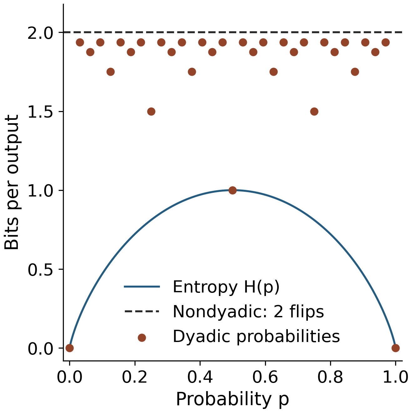
This is the average information in one output, measured in bits. It is at most one, and approaches zero for an almost deterministic coin. Why, then, does a single exact nondyadic sample still need two fair bits on average?
The decision tree must allocate whole leaves, each with probability . For one output, that indivisibility has a cost. Knuth and Yao’s bound, as stated in 2, places the optimum for a finite distribution between its entropy and its entropy plus two bits.
Reproduce this figure
tar -xf coin-sampling-gen_figures.tar && cd coin-sampling-gen_figures/coin-sampling && uv run --locked gen_figures.pyRequires uv and Python 3.12; the locked packages download on first run.
Now treat independent Bernoulli outputs as one outcome from a distribution on strings. Their total entropy is . Applying the same theorem to that product distribution gives
The expected number of fair bits per output therefore lies between and . For , entropy is about bits; with blocks of 100, the theorem guarantees a rate below bits per output. Calling the one-coin procedure 100 times still costs 200 bits on average. Batching changes the sampler.
This is a theoretical bit-cost statement. Constructing the product distribution’s decision tree may be expensive, and the theorem is not a recommendation to materialize possibilities.
The connection to compression is more direct than a shared entropy formula. A compressor gives likely strings short descriptions. A sampler allocates more random-bit paths to likely strings. Arithmetic coding expresses both through intervals: encoding narrows an interval according to observed symbols; decoding random bits selects symbols according to the interval lengths. That exact interpretation assumes exact interval boundaries; finite-precision coding implementations may round them.4
The first-heads trick is a small instance of that correspondence. Each binary digit says whether its share of random-bit space belongs to success. Grouping outputs lets those shares be allocated more efficiently.
# Reproducing the calculations
The reproduction bundle contains the integer samplers and exact decision-tree checks. It explores every rational input with and through depth 12, comparing leaf masses and unfinished mass with the target probabilities and the optimal tail bound. These are exact rational calculations, so the checks do not depend on simulation noise. It also checks recycled dice and bounds the sampler’s success probability by accounting for every still-unfinished bit prefix. The figure source downloads include the dependency lockfile and shared plotting helper.
# References
[1] Jérémie Lumbroso (2013). Optimal Discrete Uniform Generation from Coin Flips, and Applications. Section 1 and Appendix B. ↩
[2] Feras A. Saad, Cameron E. Freer, Martin C. Rinard, and Vikash K. Mansinghka (2020). The Fast Loaded Dice Roller. Section 2, Theorem 2.1, states the Knuth–Yao result from The Complexity of Nonuniform Random Number Generation (1976). ↩
[3] Python documentation. random: Generate pseudo-random numbers. Precision and distribution of random(). ↩
[4] Paul G. Howard and Jeffrey Scott Vitter (1992). Practical Implementations of Arithmetic Coding. Arithmetic coding as a bridge between random bits and prescribed distributions. ↩
[5] Philippe Flajolet, Maryse Pelletier, and Michèle Soria (2011). On Buffon Machines and Numbers. SODA 2011, pp. 172–183, especially Section 2.2. ↩