Common on the board, rare in English

November 26, 2016revised September 20, 2026

Toea looks like a good Boggle word. It uses four common letters, appears in the selected dictionary, and is uncommon in general English. But those facts do not yet tell us whether memorizing it earns points. The board has to contain it, the player has to notice it under time pressure, and no opponent can write it down.

That gives four separate measurements:

1. Board probability: $p_{\mathrm{board}}(w)$, the probability that at least one valid path spells $w$.
2. Solo opportunity: official points times board probability.
3. Findability: the probability that a particular player notices $w$, conditional on its presence.
4. Uncancelled score: findability after accounting for every opponent who may find the same word.

The first two can be simulated. The last two need people.

# What counts as a Boggle word

Classic Boggle has 16 cubes in a 4-by-4 grid. Consecutive letters must be horizontally, vertically, or diagonally adjacent, and a cube may appear only once in a path. A word must contain at least three letters. The Qu face contributes both letters while occupying one cube.1

The official score is:

In multiplayer play, a word found by two or more players is crossed off every list. Finding the same word along two paths does not score twice. These rules matter: raw board frequency is neither expected score nor competitive value.

The analysis uses the 16 cube faces transcribed in its generator and the ENABLE word list in games/boggle.2 The rules document establishes play rules, not this particular cube inventory, so these probabilities describe the modeled set rather than every physical edition of Boggle. ENABLE is a permissive general word-game lexicon, not an official Hasbro tournament dictionary. Any real game still needs an agreed dictionary.

# A tile is not always a character

A direct board representation stores the special face as one tile:

('h', 'i', 'm', 'n', 'qu', 'u')

The original notebook then built a character-keyed trie, but looked up the whole tile as one key:

letter = board[i][j]
if letter in node:
    node = node[letter]

A character-keyed trie contains a q edge followed by a u edge; it contains no qu edge. Looking up the whole tile as one key silently rejects every Q-word. Storing the face as plain q makes the opposite mistake by allowing Q without its mandatory U.

The corrected solver consumes every character printed on a tile before moving to a neighboring cube:

def advance(node, tile):
    for character in tile:
        node = node.get(character)
        if node is None:
            return None
    return node

The path still marks only one cube as visited, while its spelling grows by two letters. That also makes the official length score come out correctly.

# Sampling boards

If the cubes are treated as labeled, there are

$$16!\,6^{16} \approx 5.9 \times 10^{25}$$

position-and-face outcomes. Duplicate faces and symmetries mean fewer distinct visible grids, but exact enumeration is impractical for estimating common-word probabilities.

For a fixed word $w$, let $X_{b,w}=1$ when board $b$ contains at least one valid path spelling $w$, and $X_{b,w}=0$ otherwise. Across $n$ independently generated boards,

$$\hat p_w=\frac1n\sum_{b=1}^{n}X_{b,w}$$

estimates the board probability $p_w$. Hoeffding’s inequality gives5

This is a concentration bound: averages of independent yes-or-no trials stay close to their true probability. Here each $X_{b,w}$ is one such trial, so the bound turns a desired error margin and failure probability into a board count:

$$\Pr\!\left(\left|\hat p_w-p_w\right|>\varepsilon\right) \leq 2e^{-2n\varepsilon^2}.$$

To make the right side at most $\delta$, it is enough to choose

$$n\geq\frac{\log(2/\delta)}{2\varepsilon^2}.$$

Setting $\varepsilon=0.01$ and $\delta=0.1$ gives $n\geq14{,}979$. That is a 90% guarantee for one fixed word chosen before the boards are inspected. For $K$ fixed words, a simultaneous union-bound guarantee replaces $\delta$ by $\delta/K$. A list selected after inspecting thousands of words instead needs simultaneous control or an independent holdout sample.

The first table below includes ordinary 95% Wilson intervals for the displayed word probabilities. Those are marginal binomial intervals. They do not adjust for selecting the displayed words from the same simulation, and neither the intervals nor Hoeffding’s bound claim that a near-tied top-20 list is exactly ordered. The figure’s frontier gets a separate check: it is computed independently in each half of the simulation, and only words on both frontiers receive the solid highlight.

The generator runs 15,000 boards with seed 20161126. It verifies the SHA-256 digest of the dictionary file, so a changed word list cannot silently change the result.

The figure’s source bundle also regenerates the tables and prints the selection diagnostics.

# What appears

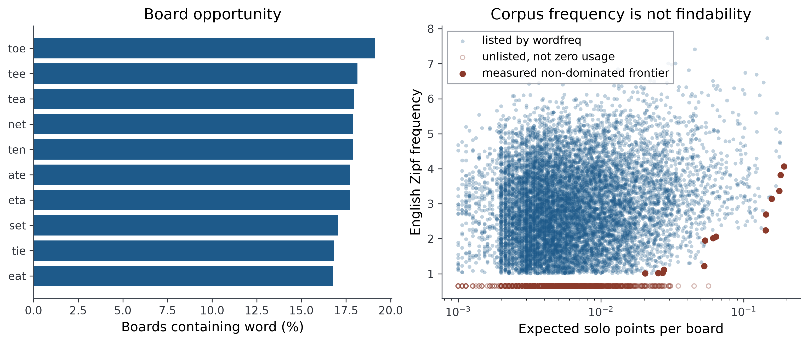
With the official three-letter minimum, short words dominate:

Filtering to words of at least four letters produces a different but still tightly clustered list:

The reproducible result is the estimated probability and its sampling uncertainty, not which near-tied word happens to finish first.

# Opportunity is not value

For solo play, a measurable first approximation is

$$O(w)=s(w)\,p_{\mathrm{board}}(w),$$

where $s(w)$ is the official point value. This is the expected number of points made available by the word per random board, assuming a perfect solver. It says nothing about whether a human finds the word.

TF-IDF is not the right name for a board-frequency ranking: there are no documents and no document frequencies. Multiplying board appearance by a decreasing function of corpus token count is a custom heuristic. Assigning a missing corpus entry the smallest observed count would also make “absent from this corpus” numerically identical to “maximally obscure,” even though absence can mean a spelling, tokenization, coverage, or stemming mismatch.

The figure keeps the axes separate. The horizontal axis is measured solo opportunity. The vertical axis is wordfreq 3.1.1’s English Zipf estimate, an aggregate over several processed text sources rather than a direct count from one corpus.3 Points must appear on at least 15 simulated boards. The solid rust points are non-dominated in both independent 7,500-board halves under the same rule: at least eight appearances, positive wordfreq frequency, and at least 0.003 expected solo points per board. Their plotted coordinates pool all 15,000 boards; the split only checks whether the frontier membership recurs. Open rust circles are words below wordfreq’s wordlist cutoff; they sit on an artificial baseline at 0.65 so the package’s zero default is not presented as zero English usage.

Reproduce this figure

Download source bundleextract, then runtar -xf boggle-words-gen_boggle_opportunity.tar && cd boggle-words-gen_boggle_opportunity/boggle-words && uv run --locked gen_boggle_opportunity.py

Requires uv and Python 3.12; the locked packages download on first run.

The Boggle dictionary is not bundled: set BOGGLE_DICTIONARY to the pinned file for offline use, or allow the script to download and verify it.

Individual files:gen_boggle_opportunity.pylockfilefigure_quality.py

Eight illustrative, hand-selected low-corpus-frequency four-letter words occupy an interesting part of that space. This is not a top-eight ranking:

Corpus frequency is not familiarity, and familiarity is not timed discovery. Word-prevalence norms ask people whether they know a word and cover 61,858 English lemmas from more than 220,000 participants; they predict recognition beyond corpus frequency.4 Even those norms would measure knowledge, not whether a winding Boggle path is noticed within the round’s time limit.

# The multiplayer quantity

Let $q_0(w)$ be the focal player’s probability of finding $w$ when it is present, and let $q_j(w)$ be the same probability for opponent $j$. If those probabilities are treated as board-invariant and the players’ find events are independent conditional on presence, the expected uncancelled contribution is

$$\boxed{ \mathbb{E}[\mathrm{score}(w)] =s(w)\,p_{\mathrm{board}}(w)\,q_0(w) \times \prod_{j=1}^{m}\left(1-q_j(w)\right) }$$

For one opponent, the conditional scoring event is “the focal player finds the word and the opponent does not,” with probability $q_{0}(w)(1-q_{1}(w))$. Multiplying the not-found factors gives the displayed formula for $m$ opponents.

This is an intentionally coarse approximation. Path geometry, alternate paths, and distracting words make findability vary from board to board; players can be independent once a board is fixed yet dependent after those boards are averaged. With board-level observations and conditional player independence, the unconditional quantity is $s(w)\mathbb{E}_{B}[I_{w}(B)q_{0}(B,w)\prod_{j}(1-q_{j}(B,w))]$, where $I_{w}(B)$ says that board $B$ contains $w$. For example, if the word occurs on every board, half the boards are easy enough that both players find it, and on the other half neither does, the marginal find probabilities are both one half. The displayed approximation assigns $s(w)/4$, but the uncancelled score is zero. Players also share vocabulary, visual biases, and training histories. A hierarchical model could represent both sources of dependence.

# The experiment still needed

A useful memorization study would randomize players to a taught list and a matched control list. The lists should be matched on length, board probability, path geometry, and baseline word prevalence. On unseen boards, record:

• whether each present target word was found;
• time to first find;
• its path shape and number of alternate paths;
• whether an opponent also found it;
• retention after a delayed session.

The treatment effect estimates how much teaching changes $q_0(w)$. Multiplayer rounds estimate cancellation. Until those measurements exist, the current evidence supports a map of promising words to test, not a declaration that toea is worth memorizing.

# References

[1] Hasbro, Boggle Instructions, classic 4-by-4 rules: adjacency, no cube reuse, duplicate cancellation, Qu counting as two letters, and the 1/2/3/5/11 scoring schedule. ↩

[2] Wallace, H. (2016). Common Words in Boggle notebook, first committed November 26, 2016. The analysis pins enable1.txt from commit 8407a721b8b904b861b1dc71233cc8370dbe6673, SHA-256 a392640f14602fcbb36779eb6671d170260c06d43f41c16383e7f0e35b221b4a. ↩

[3] Speer, R. (2022). wordfreq v3.1.1. The generator pins this version. Its zero default means that a word is below the selected wordlist’s cutoff or absent from it; it does not establish zero English usage. ↩

[4] Brysbaert, M., Mandera, P., McCormick, S. F. & Keuleers, E. (2019). “Word prevalence norms for 62,000 English lemmas.” Behavior Research Methods 51(2), 467–479. ↩

[5] Hoeffding, W. (1963). “Probability Inequalities for Sums of Bounded Random Variables.” Journal of the American Statistical Association 58(301), 13–30. ↩