Passive WiFi Channel Hopping as Active Sensing
Published June 26, 2023 · Revised July 24, 2026
A radio can listen on only one WiFi channel at a time. An adaptive strategy is to spend more time where it hears more packets, but packet volume is not the same objective as discovering short-lived devices or attacks. A useful model is active sensing: define the events that matter, the listening intervals that catch them, and a revisit constraint. Bandit algorithms can then allocate the remaining time without pretending that best-arm regret is a coverage guarantee.
A monitor-mode WiFi radio faces a scheduling problem. At any instant it can capture one channel and miss every other one. Should it sweep uniformly, dwell where traffic is heavy, or learn a schedule online?
The answer depends on what “good monitoring” means. Maximizing captured packets, discovering access points, catching a brief deauthentication burst, and bounding the time until every channel is revisited are different objectives. A policy can be excellent at one and poor at another.
# The Physical Setting
In monitor mode, an interface can receive 802.11 frames without joining the network. Radiotap metadata may preserve the tuned frequency, signal strength, rate, and other receiver details, but it does not remove the tuning constraint: a narrowband radio still misses frames sent outside the channel it is currently monitoring.
The available channel set depends on regulatory domain, band, channel width, and hardware. The 2.4 GHz band has a small, partly overlapping set; 5 and 6 GHz offer many more possible center frequencies. Wider bandwidth can observe more spectrum at once but changes sensitivity, decoding, and hardware requirements. For scheduling, the correct arm set is therefore the set the specific radio can legally tune and decode, not an abstract list of channel numbers.
# What a Channel Hop Can Measure
Suppose the radio chooses channel for dwell interval . It observes packets on that channel during that interval. Two useful summaries are:
and
where an event has a channel, start time, end time, and perhaps a value . The first quantity is packet volume. The second says whether the monitor caught a particular event under an idealized continuously observable-event model. A packet-level event also requires the radio to receive and decode an event-bearing frame during the overlap; temporal overlap alone is not enough.
These observables support different goals:
| Goal | Measurement |
|---|---|
| Capture traffic volume | packets or bytes captured |
| Inventory persistent APs | probability of at least one beacon per AP |
| Catch transient activity | fraction or value of events detected |
| Bound discovery delay | maximum or quantile revisit time |
| Reconstruct a trace | contiguous capture and frame-sequence completeness |
A packet-rate bandit directly addresses only the first row. Packet rate can be a useful predictor for the others, but the connection is an assumption to test, not a theorem inherited from bandit regret.
# Existing Schedules and Earlier Adaptive Sampling
Production tools expose the tradeoff rather than eliminate it. Kismet’s documentation describes a compromise between changing channels to learn about the wider environment and remaining on one channel for complete capture. Its default five hops per second is a practical choice relative to APs beaconing about ten times per second; the documentation does not claim an independent-Poisson capture guarantee. Beacon transmissions are scheduled around a target beacon interval, so is not automatically the right per-visit model.
airodump-ng uses an interleaved channel order rather than an ascending
sweep. Its 14-channel sequence at the source revision inspected
here,
{1,7,13,2,8,3,14,9,4,10,5,11,6,12}, spreads many consecutive frequencies
apart, but it is not a maximizer with minimum adjacent gap
: several adjacent differences are 5.
Adaptive channel sampling is also older than modern bandit terminology in this application. Deshpande, Henderson, and Kotz implemented and evaluated two WiFi monitoring schedules in 2006:1
- equal time on every channel;
- dwell time proportional to the frame rate observed in the previous cycle.
They made the objective application-specific, imposed a minimum interval, measured switching overhead, tested intrusion-alert capture, and recommended randomization when an attacker might learn the schedule. The contribution left for a modern treatment is therefore not “first adaptive WiFi hopping.” The remaining contribution is to separate monitoring targets, online uncertainty, constraints, and current wide-band channel counts.
Later work made the learning formulation explicit. Le, Szepesvári, and Zheng modeled passive multi-channel sniffers as a linear partial-monitoring problem with switching costs in 2014.4 Their payoff was expected distinct users detected, not raw packet count, and their block-UCB schedule used growing epochs to reduce retunes. The result is directly relevant prior art, while still relying on its own stationary payoff model.
# Packet Capture as a Bandit
For a fixed dwell duration, let the decoded frame count on channel be
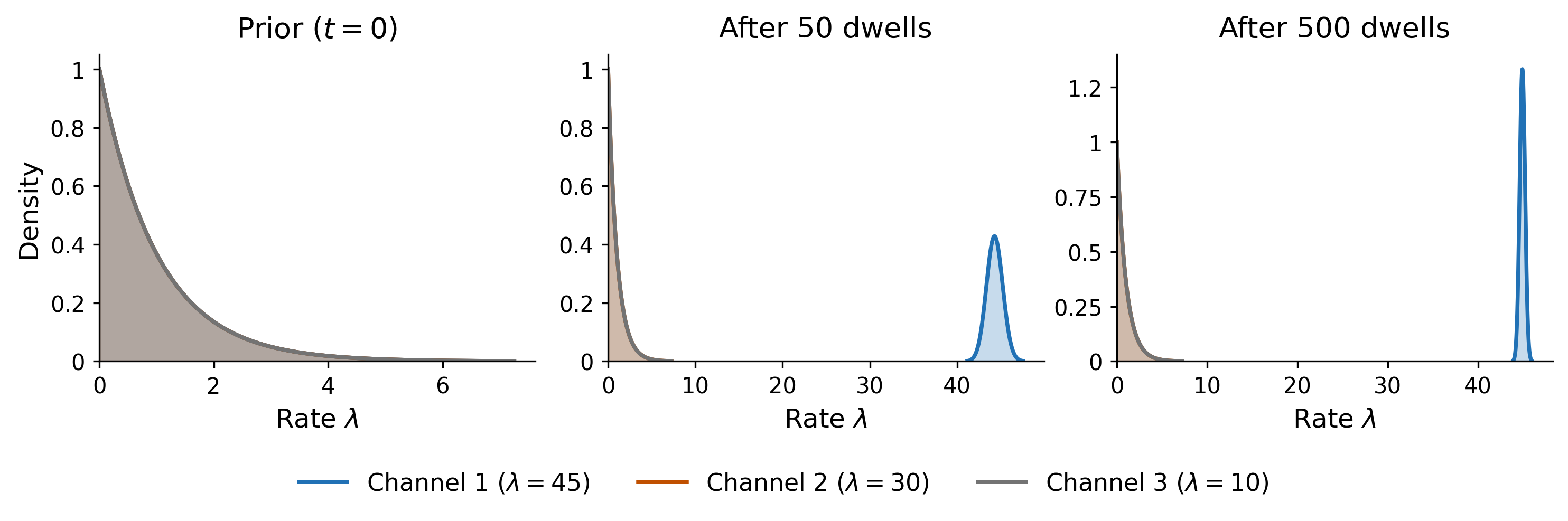
This is a useful teaching model for packet-volume allocation. A Gamma–Poisson Thompson sampler maintains
in the rate parameterization. After observing packets during one unit of exposure on channel ,
At each decision it samples one rate from every posterior and chooses the largest. For unequal dwell durations, the second update must add the exposure time rather than incrementing by one.
Reproduce this figure
For Poisson arms, a distribution-aware KL-UCB index is another appropriate choice. The Poisson divergence is
The UCB1 formula with is derived for bounded rewards on a common scale. Raw Poisson counts are unbounded and have variance that grows with their mean, so applying that formula without normalization does not inherit the UCB1 bound. Exponential-family KL-UCB or a Poisson confidence sequence is derived for this reward model.2
Under stationary independent Poisson arms, Poisson KL-UCB and Thompson sampling have asymptotic-optimality results under their respective conditions.3 6 Those results compare a learner with an oracle that always listens to the highest-rate channel. They say nothing about a quiet channel carrying the one event the operator cares about.
For equal dwell intervals, that classical packet-count regret is
where . This is a useful benchmark when captured packet volume really is the objective. It is not a universal definition of monitoring loss.
# Event Discovery Changes the Objective
Let be the events occurring during the observation horizon. A value-weighted discovery objective is
This definition exposes the assumptions a packet proxy would need:
- event arrival rates must correlate with background packet rates;
- event durations must be long relative to revisit gaps;
- decoded packet counts must be comparable across channels;
- the value must not be concentrated on rare, quiet channels.
If any of these fail, maximizing packets can reduce discovery.
# A failure pair
Consider two worlds with exactly the same background packet rates.
- In world A, important events occur in proportion to those rates.
- In world B, important events occur mostly on quiet channels.
A packet-rate learner receives the same evidence in both worlds until it catches an event, yet their optimal schedules differ. Packet counts alone do not identify the event-optimal policy.
# Coverage Is a Constraint, Not an Entropy Metaphor
A useful production policy separates a mandatory coverage layer from an adaptive allocation layer.
Suppose there are channels, each decision visits one channel, and decisions have equal duration. A maximum revisit interval is feasible only if : otherwise the pigeonhole principle leaves some channel unvisited. Begin with one coverage cycle so that every channel has a recorded visit. Thereafter, at decision :
- if any channel has not been visited for decisions, visit the most overdue channel;
- otherwise, let the adaptive packet- or event-value policy choose.
Under those capacity and initialization conditions, the rule gives a directly checkable schedule invariant:
with the boundary gaps checked separately:
over a monitoring horizon . The invariant bounds gaps between visit starts. The actual continuously unobserved time also depends on dwell length and retune time, so those quantities must be included when is translated into an event-duration guarantee. Unequal dwell times require the same feasibility check in elapsed time rather than decision counts. The constraint does not guarantee that every device is detected: an event shorter than the off-channel gap can still occur wholly between visits.
For a periodic cycle of length , one listen interval of length , and an event of length whose start phase is uniform, the probability of any overlap is
To derive it, place the listen interval at on a circle of circumference . An event beginning at phase overlaps that interval exactly when lies in the listen arc expanded backward by , namely modulo . That expanded arc has length , so dividing by gives the displayed probability.
Endpoint contact has zero probability under the continuous uniform-phase model. Consequently gives overlap probability one while still leaving one boundary phase with no positive-duration overlap. A deterministic positive-overlap guarantee requires the strict inequality . With several listen intervals per period, the eligible phases form a union of backward-expanded arcs; their overlaps must be merged rather than adding single-interval probabilities. For irregular schedules, evaluate overlap against the actual listen intervals, as the replay below does.
The weaker long-run formulation requires visit frequencies with , then optimizes the remaining allocation. A frequency floor controls average allocation but still permits arbitrarily long finite blind gaps; it is not equivalent to the maximum-revisit invariant above. This is a constrained allocation problem, not the resource-consumption model of Bandits with Knapsacks.
The public muxer 0.5.3 crate contains a
reusable version of this separation: a coverage quota can override an adaptive
router. Its quota enforces an empirical minimum sampling fraction, not the hard
maximum-revisit interval defined above. It also supplies an Exp3-IX router for
adversarial rewards. In that release, the Thompson sampler is Beta/Bernoulli,
so a WiFi Gamma–Poisson or event-value adapter would be new implementation
work rather than an existing channel hopper.
# A Controlled Replay
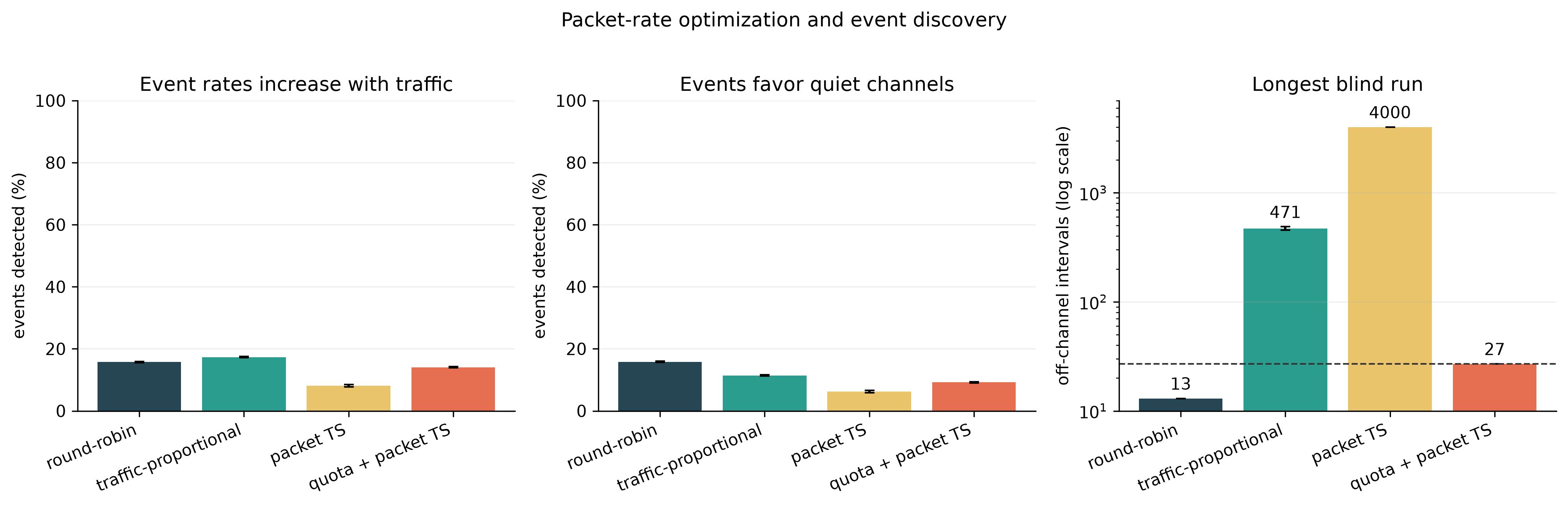
The accompanying simulation deliberately separates background packet rate from transient-event arrival rate. Four schedules receive the same packet-count process:
- round-robin;
- allocation proportional to the true packet rates;
- pure Gamma–Poisson packet Thompson sampling;
- the same sampler with a 28-decision maximum-revisit quota.
Events last a capped-geometric number of decision intervals, with a maximum of 12. In one environment event arrival rates increase with packet traffic but retain a common floor; in the other they favor quiet channels. The experiment uses 14 channels, 4,000 decisions, 200 independent runs, a fixed seed, and reports 95% normal intervals across runs. Within each run, each policy schedule is generated once and replayed against both event environments.
Reproduce this figure
The absolute percentages depend on the simulated event duration and arrival rates. The result shared by both simulated event models is structural: learning the packet-rate ranking more confidently does not reveal whether event value follows that ranking. The quota limits starvation; it cannot manufacture the missing relationship.
# Switching, Leakage, and Non-stationarity
# Switching cost
If every decision changes channel, a hop that takes milliseconds followed by a dwell of leaves the usable fraction
For an arbitrary schedule over horizon , the more general accounting is : choosing the same channel again causes no retune. The cost is both lost capture time and a reason not to switch after every small posterior fluctuation. A scheduler can charge an explicit switch penalty, batch several dwells on one channel, or optimize dwell length jointly with channel choice.
SpecWatch applies batching to adversarial spectrum misuse and proves sublinear weak regret for an EXP3-style monitor with switching costs.5 Its cognitive-radio threat model, timeslots, and multi-radio actions are not direct validation for passive 802.11 capture; they are a concrete example of matching the learning model to a schedule-aware environment.
# Adjacent-channel observations
Channel overlap can provide side observations, but RF power leakage and decoded frame counts are not interchangeable. An interference factor measured from received power does not by itself define a linear mixture of successfully decoded packets. Nor can one scalar observation from a single tuned channel be inverted into a full vector of channel rates.
A defensible correction requires calibration data:
- transmit known traffic on source channel ;
- tune the monitor to channel ;
- estimate the probability that a frame from is detected and decoded;
- repeat across hardware, bandwidths, power, and environment.
The result is an observation model , not necessarily a fixed invertible matrix. When calibrated side observations are reliable, a structured or graph-feedback bandit can use them. Otherwise, retain source channel metadata on decoded frames and avoid deconvolution claims.
# Non-stationarity
Traffic and event rates change. Sliding windows, discounted posteriors, and change-point-triggered resets are possible responses, but each defines a timescale. A policy tuned to seconds will react differently from one tuned to a shift change. Report that timescale and test it against multiple drift speeds; “non-stationary” alone is not a model.
# Choosing a Schedule
| Monitoring requirement | Starting policy |
|---|---|
| Persistent AP inventory | round-robin or PSC-aware sweep with explicit revisit bound |
| Maximum packet volume | traffic-proportional allocation, Poisson KL-UCB, or Gamma–Poisson Thompson sampling |
| Short rare events on unknown channels | randomized coverage schedule with a tight revisit bound |
| Events correlated with known context | constrained contextual or event-value bandit |
| Complete protocol trace | dedicate a radio; hopping is the wrong architecture |
Multiple radios and wideband capture change the feasible set. Kismet can divide channel lists across interfaces; a dedicated radio per important channel removes the scheduling uncertainty there. In 6 GHz, Preferred Scanning Channels and Reduced Neighbor Reports provide context for discovery, but they do not imply that non-PSC activity is irrelevant to a security monitor.
The implementation question is therefore not “which bandit wins?” It is:
What event or trace property must be observed, how long does it remain observable, and what blind interval can the application tolerate?
Once those are explicit, a bandit can allocate the remaining time adaptively. Otherwise, logarithmic regret may optimize a different objective from the monitoring one.
# References
[1] Deshpande, U., Henderson, T., & Kotz, D. (2006). “Channel Sampling Strategies for Monitoring Wireless Networks.” WiNMee. ↩
[2] Garivier, A. & Cappé, O. (2011). “The KL-UCB Algorithm for Bounded Stochastic Bandits and Beyond.” COLT. Poisson and other exponential-family divergences are treated in the model-specific extension. ↩
[3] Lai, T. L. & Robbins, H. (1985). “Asymptotically Efficient Adaptive Allocation Rules.” Advances in Applied Mathematics, 6(1), 4–22. ↩
[4] Le, T. M., Szepesvári, C., & Zheng, R. (2014). “Sequential Learning for Multi-Channel Wireless Network Monitoring With Channel Switching Costs.” IEEE Transactions on Signal Processing, 62(22), 5919–5929. ↩
[5] Li, M., Yang, D., Lin, J., Li, M., & Tang, J. (2018). “SpecWatch: A Framework for Adversarial Spectrum Monitoring with Unknown Statistics.” Computer Networks, 143, 176–190. ↩
[6] Korda, N., Kaufmann, E., & Munos, R. (2013). “Thompson Sampling for 1-Dimensional Exponential Family Bandits.” NeurIPS. ↩